Predicting Level of Acceptability of Cars using Machine Learning
Summary
In this project, we attempt to predict the level of acceptability of cars by building a machine learning model in Python (Van Rossum and Drake 2009). The acceptability levels include four class labels: unacc (unacceptable), acc (acceptable), good, and vgood (very good). We use a data created by the efforts of M. Bohanec in the late 1980s. It is sourced from the UCI Machine Learning Repository and is publicly available for research (Bohanec 1988). Every feature and target in this dataset is encoded by one-hot encoder for data analysis. To choose the best model for this task, we utilised several common machine learning models, and found out that the SVM RBF classifier achieved the best train and cross-validation scores, with a test accuracy of 0.952. The SVM RBF model also showed exceptional ability in determining the acceptability of cars as seen in accuracy. Because we see that there is a class imbalance on the dateset, we calculate the f1 score to test if our model has good performance. With a f1 score of 0.99 on test data, we justify that the model performs well on unseen data, even with a class imbalance. This makes the SVM RBF model a solid choice for this project. By looking deep into the performance of model on difference classes, we see the model performs exceptionally well overall, with near-perfect scores across all metrics. However, class good has a slight recall issue, indicating some instances of this class are being missed. A confusion matrix with cross validation is brought to further visualize what is happening.
Introduction
The Car Evaluation Dataset was created as part of efforts to understand the factors that affect the acceptability of cars among consumers. “Acceptability” is categorized as a categorical variable with four levels; “Unacceptable”, “Acceptable”, “Good”, and “Very Good.” The factors affecting acceptability include buying price of a car, maintenance costs, passenger and luggage capacity, and safety. A consumer’s decision to purchase a car is influenced by the acceptability of the car. The goal of this project is to develop a machine learning model that can evaluate the quality of a car based on its attributes to help buyers make a more informed decision for their next car purchase. Due to many factors determining the condition of a car, this is not an easy decision for consumers to make on their own.
Methods
Data
The dataset that was used in this project is of Car Evaluation Database (Bohanec 1988) created by the efforts of M. Bohanec in the late 1980s. It is sourced from the UCI Machine Learning Repository and is publicly available for research.
Each row in the dataset details a car’s attributes (each feature is of categorical data type with several levels), which includes:
- Buying price:
low,med,high,vhigh
- Maintenance cost:
low,med,high,vhigh
- Number of doors:
2,3,4,5more
- Seating capacity:
2,4,more
- Boot size:
small,med,big
- Safety rating:
low,med,high
Each row in the dataset details a car’s attributes (features) and its acceptability (target variable). The target variable is categorized into four class labels:
unacc: Unacceptable. Cars that fail to meet basic criteria.
acc: Acceptable. Cars that meet minimum requirements.
good: Good. Cars that exceed average standards in some aspects.
vgood: Very good. Cars that meet the highest standards.
Exploratory Data Analysis
Exploratory data analysis was carried out on the train dataset.
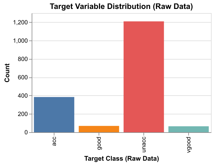
To assess the balance of target classes in the dataset, the distribution of the target variable was visualized (see Figure 1). We can see the dataset has a significant class imbalance which is the unacceptable class. This imbalance can affect model performance:
- Models may overpredict the
unacceptableclass and fail to identify minority classes (good,vgood).
- It could be high simply by predicting the majority class, so accuracy may be misleading. We can consider metrics like Precision, Recall, and F1-score.
This imbalance may require further handling. For example, oversampling, undersampling, or class-weighted loss functions during training.

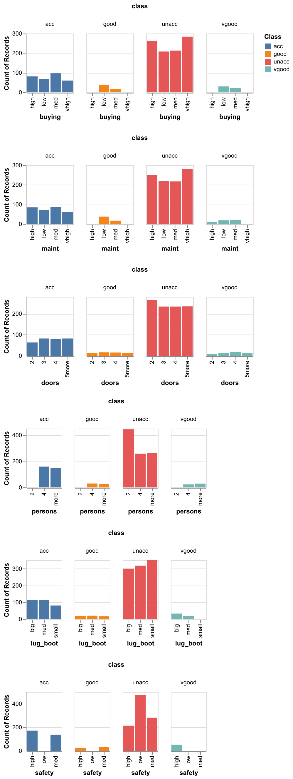
From Figure 2, we can see the counts of records by target and category was visualised to gain a better idea of the dataset.

Through this analysis, we can see that examples with target class unacceptable represent a large proportion of the dataset.
Preprocessing of Dataset for Machine Learning
We preprocess the dataset to prepare it for machine learning:
- Transform categorical features using
OrdinalEncoderfrom scikit-learn - Split the dataset into training and testing sets
Model Selection
The core of this project is choosing the appropriate machine learning model. Thus, several machine learning models from scikit-learn (Pedregosa et al. 2011) will be evaluated using cross-validation. The models evaluated are:
DummyClassifier(Dummy), which serves as a baseline to compare the performance of other models,DecisionTreeClassifier(Decision Tree),KNeighboursClassifier(KNN),SVCwith RBF kernel (SVM RBF),- Naive Bayes using
MultinomialNB(Naive Bayes), and LogisticRegression(Logistic Regression).
| Model | Mean train score | SD train score | Mean CV score | SD CV score |
|---|---|---|---|---|
| Dummy | 0.7 | 0 | 0.7 | 0.001 |
| Decision Tree | 1 | 0 | 0.97 | 0.009 |
| KNN | 0.97 | 0.003 | 0.943 | 0.011 |
| SVM RBF | 0.971 | 0.004 | 0.952 | 0.018 |
| Naive Bayes | 0.711 | 0.002 | 0.708 | 0.004 |
| Logistic Regression | 0.838 | 0.007 | 0.834 | 0.019 |
The results of the model selection is shown in Table 1. According to the results, SVM RBF achieved high train and cross-validation scores of 0.971 and 0.952 respectively, suggesting it is the best model for generalising unseen data.
While the Decision Tree model yielded the best train and cross-validation scores, the perfect train score suggests that the model has overfitted to the data. Therefore, we will be using SVM RBF for this project.
Model Optimization
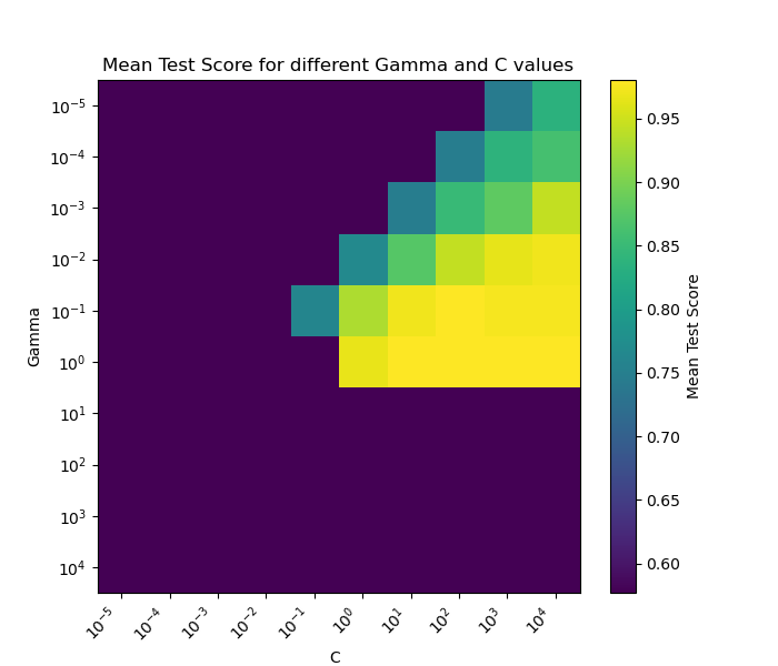
With the best model identified, the next step was to improve its performance through hyperparameter optimization. Using RandomizedSearchCV, a range of values for the SVM’s hyperparameters C and gamma were explored. The range of hyperparameters was chosen to cover a range of possibly useful hyperparameter values, which are commonly used in hyperparameter optimization for SVM classifier (Developers 2024). This approach allowed for an efficient and thorough search across the parameter space, and results in an optimal esitimator to use. We use f1 weighted score to tune because of a multiclass dataset.
The visualizations are below, including a heatmap (Figure 3) of test scores obtained during hyperparameter optimization. This interpretability aids in understanding which parameters are most critical and how sensitive the model is to these settings.

We observed that the best hyperparameter of C and gamma are 100.0 and 0.1 respectively. All categorical features were passed through OrdinalEncoder prior to model fitting. The Python programming language (Van Rossum and Drake 2009) and the following Python packages were used to perform the analysis: numpy (Harris et al. 2020), Pandas (McKinney 2010), matplotlib (Hunter 2007), scikit-learn (Pedregosa et al. 2011). The code used to perform the analysis and create this report can be found here: https://github.com/UBC-MDS/Car_Evaluation_Analysis/blob/main/scripts
Results & Discussion
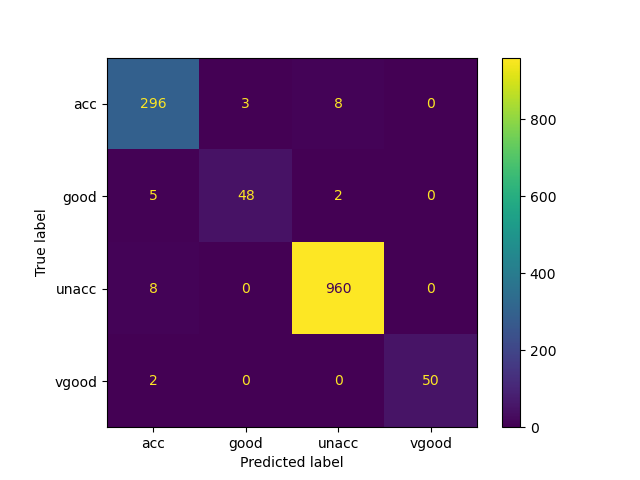
After performing hyperparameter optimization, the SVM RBF model manage to achieve the best f1 score of 0.99 on the test data. This suggests the model has been generalised well, with high scores on both the train and test sets. Let’s have a look at the classification report Table 2. It has a balanced performance across precision, recall, and F1-scores for each class. The weighted average metrics further confirm the robustness of the model. The weighted average F1-score 0.991 reflects balanced performance even with class imbalance. However, slightly lower recall for class “good” (0.857) suggests some misclassification, which could be improved with better feature engineering, or can be improved by increasing the data points.
| class | precision | recall | f1-score | support |
|---|---|---|---|---|
| acc | 0.962 | 1 | 0.981 | 77 |
| good | 1 | 0.857 | 0.923 | 14 |
| unacc | 1 | 0.996 | 0.998 | 242 |
| vgood | 1 | 1 | 1 | 13 |
| accuracy | 0.991 | 0.991 | 0.991 | 0.991 |
| macro avg | 0.991 | 0.963 | 0.975 | 346 |
| weighted avg | 0.992 | 0.991 | 0.991 | 346 |
Below is a confusion matrix from cross validation (Figure 4), we can visualize how model performs specifically on each classes.

To further improve the model’s utility, several changes can be made. One such change is feeding the model with features that are not just categorical. Instead, for features such as buying price, maintenance cost and safety features, numeric data should be collected. At the same time, more features can be included, such as the type of car and and fuel efficiency ratings.
By allowing the model to take in more complex data, this may allow the model to make more accurate predictions to let customers make a more informed choice when purchasing a new car.