DSCI_531_viz-1
Lecture 2 Worksheet
suppressPackageStartupMessages(library(tidyverse))
library(gapminder)
students <- as_tibble(HairEyeColor) %>%
    uncount(n)
Note: students contains 592 observations of Hair, Eye, and Sex:
students %>%
    sample_n(10)
## # A tibble: 10 x 3
##    Hair  Eye   Sex
##    <chr> <chr> <chr>
##  1 Blond Blue  Female
##  2 Brown Blue  Male
##  3 Brown Brown Female
##  4 Brown Brown Male
##  5 Black Blue  Male
##  6 Brown Blue  Male
##  7 Brown Brown Female
##  8 Brown Brown Female
##  9 Brown Blue  Female
## 10 Black Brown Male
Finish 1- and 2- variable plots from last time
Bar plots
Uses of bar plots:
- Estimate probability mass functions / view frequencies of categories
- One categorical variable.
- Compare a single numeric response corresponding to different categories.
- One categorical, one (unique) numeric variable.
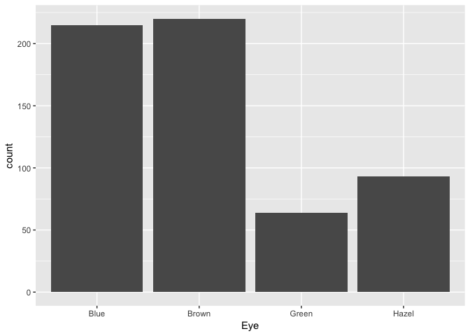
What is the distribution of eye colour in students?
ggplot(students, aes(Eye)) +
    geom_bar()
| Grammar Component | Specification |
|---|---|
| data | students |
| statistical transform | count |
| aesthetic mapping | x=Eye; y=count |
| geometric object | Bars |
| scale | Linear count |
| coordinate system | Rectangular/Cartesian |
| facetting | None |
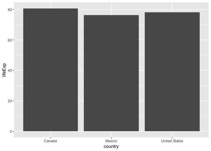
How does the life expectancy of Canada, USA, and Mexico compare in 2007?
(small_gap <- gapminder %>%
     filter(country %in% c("Canada", "United States", "Mexico"),
            year == 2007) %>%
     select(country, lifeExp))
## # A tibble: 3 x 2
##   country       lifeExp
##   <fct>           <dbl>
## 1 Canada           80.7
## 2 Mexico           76.2
## 3 United States    78.2
ggplot(small_gap, aes(x=country, y=lifeExp)) +
    geom_col()
| Grammar Component | Specification |
|---|---|
| data | students |
| statistical transform | none |
| aesthetic mapping | x=country, y=lifeExp |
| geometric object | Bars |
| scale | Linear |
| coordinate system | Rectangular/Cartesian |
| facetting | None |
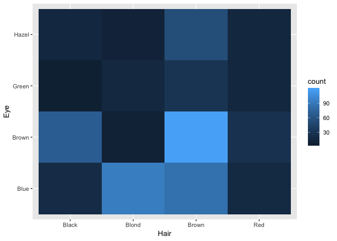
Heatmaps
Use of heatmaps: show dependence amongst two categorical variables.
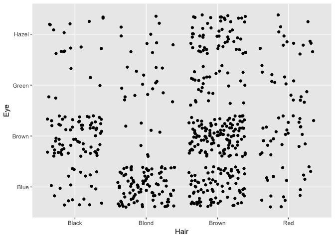
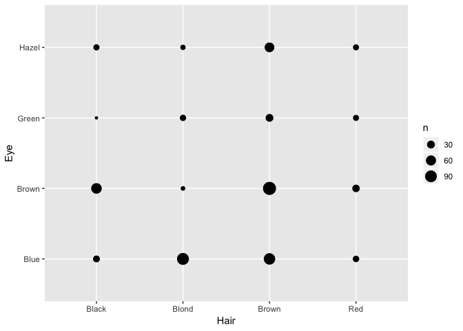
Example: Dependence amongst hair colour and eye colour in the students data.
- Points? Jitter? No.
geom_count()?geom_bin2d()!
heat <- ggplot(students, aes(Hair, Eye))
heat + geom_jitter()
heat + geom_count()
heat + geom_bin2d()
Fill in the grammar components:
| Grammar Component | Specification |
|---|---|
| data | students |
| statistical transform | count |
| aesthetic mapping | x=Hair, y=Eye; colour=count |
| geometric object | rectangles/squares |
| scale | Linear count |
| coordinate system | Rectangular/Cartesian |
| facetting | None |
Three+ Variable Plots
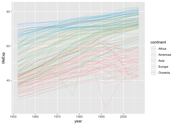
Time/Line Plots
Uses of time/line plots:
- Visualize trends of a numeric variable over time.
Plot life expectancy over time for each country in gapminder.
ggplot(gapminder, aes(year, lifeExp)) +
    geom_line(aes(group=country, colour=continent), alpha=0.2)
| Grammar Component | Specification |
|---|---|
| data | gapminder |
| statistical transform | none |
| aesthetic mapping | x=year, y=lifeExp, group=country, colour=continent |
| geometric object | line |
| scale | x and y both linear |
| coordinate system | Rectangular/Cartesian |
| facetting | None |
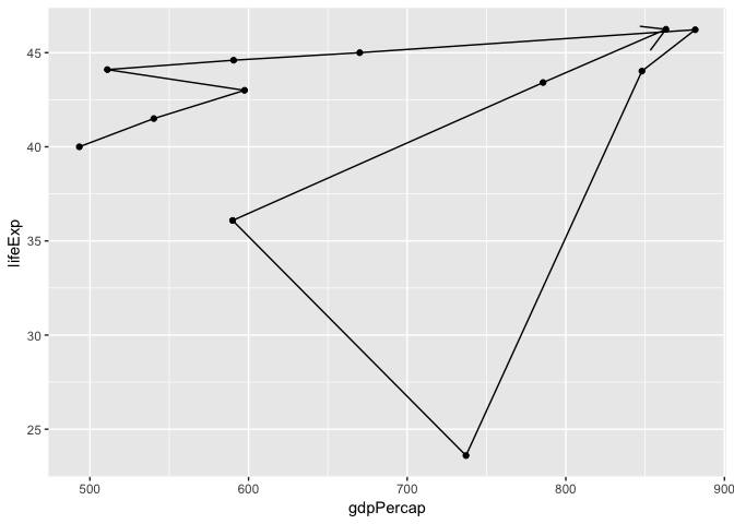
Compare to path plots, for which the order matters:
Add to the following scatterplot to see how Rwanda’s life expectancy and GDP per capita evolved over time:
gapminder %>%
    filter(country == "Rwanda") %>%
    arrange(year) %>%
    ggplot(aes(gdpPercap, lifeExp)) +
    geom_point() +
    geom_path(arrow=arrow())