Outline
- Thinking About of Probability
- Probability Distributions
- Measures of Central Tendency and Uncertainty
1. Thinking About of Probability
- Probability is recurring throughout different Data Science-related topics.
- In MDS, you will find it in either the Statistics or Machine Learning courses.
1.1. Defining Probability
Let \(A\) be an event of interest, its probability is denoted as \[P(A) = \frac{\text{Number of times event $A$ is observed}}{\text{Total number of events observed}}\]
as the total number of events observed goes to infinity.
The Coin Toss
- Frequentist Statistics is the mainstream approach we learn in introductory courses.
- Let us illustrate the frequentist paradigm idea with the typical coin toss example.
System Insights
The coin toss represents our system for which we assume two possible random outcomes:
\[\begin{gather*}
H = \{ \text{Getting heads} \} \\
T = \{ \text{Getting tails} \}.
\end{gather*}\]
Our system has the following parameters of interest:
\[\begin{gather*}
P(H) = \text{Probability of getting heads} \\
P(T) = \text{Probability of getting tails}.
\end{gather*}\]
Probabilistic Inquiries
Suppose this coin is unfair, i.e., \[P(H) \neq P(T) \neq \frac{1}{2};\]
and we want to estimate these two unknown probabilities!
Now, think about the following questions:
- How would you estimate these two unknown probabilities?
- What are the characteristics of these two estimated probabilities?
1.2. Calculating Probabilities using Laws
- Let us start with two fundamental laws that will allow us to exercise our probabilistic reasoning:
- Law of Total Probability.
- Inclusion-Exclusion Principle.
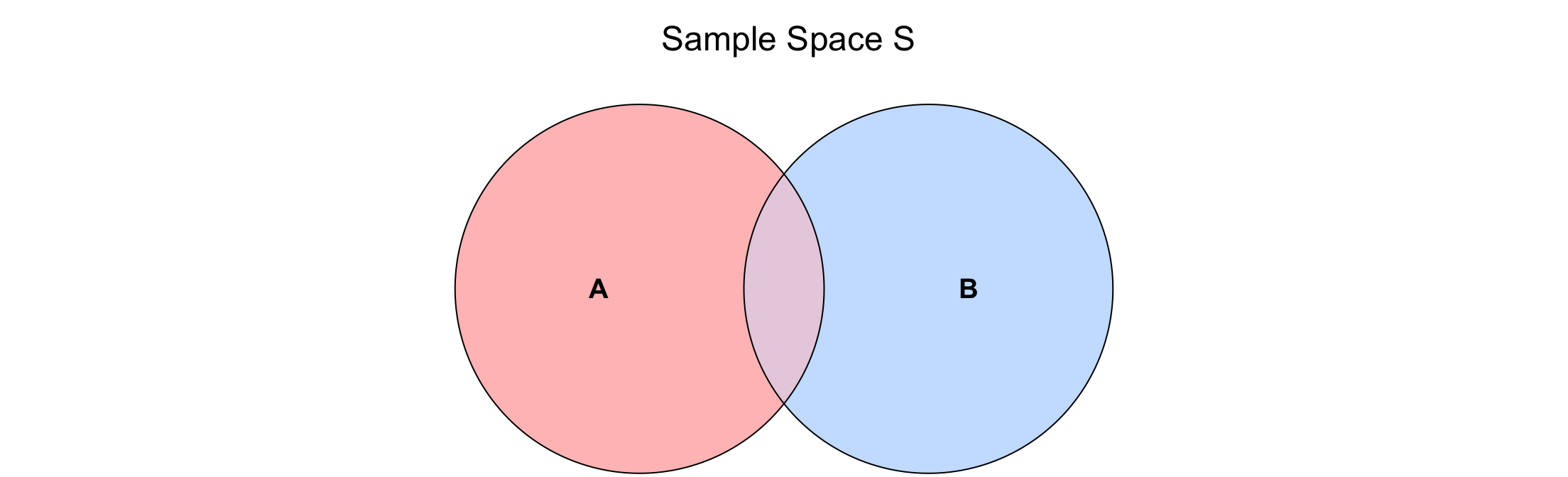
Sample Space (\(S\))
- It is the collection of all the possible outcomes of a random process or system.
- Each one of these outcomes has a probability associated with it.
- Note that \[P(S) = 1.\]
Law of Total Probability
- Breaks down the sample space \(S\) of a random process or system into disjoint parts.
- We can obtain specific probabilities based on sample space partitions.
Now, think about the following questions:
- Are there any other items possible? Why or why not?
- What is the probability of getting something other than a coin?
Inclusion and Exclusion Principle
- Let \(A\) and \(B\) be two events of interest in the sample space \(S\): \[P(A \cup B) = P(A) + P(B) - P(A \cap B).\]
Extension to Three Events
- Let \(A\), \(B\), and \(C\) be three events of interest in the sample space \(S\): \[\begin{align*}
P(A \cup B \cup C) &= P(A) + P(B) + P(C) - P(A \cap B) - P(B \cap C) \\
& \qquad - P(A \cap C) + P(A \cap B \cap C)
\end{align*}\]
Now, let us answer the following questions:
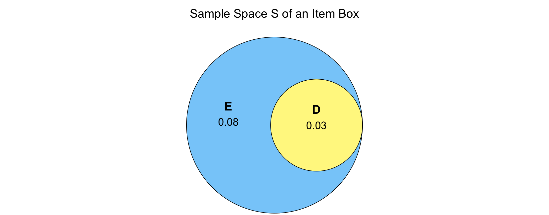
- Using the below table, what is the probability of getting an item with an explosion combat type (event \(E\))?
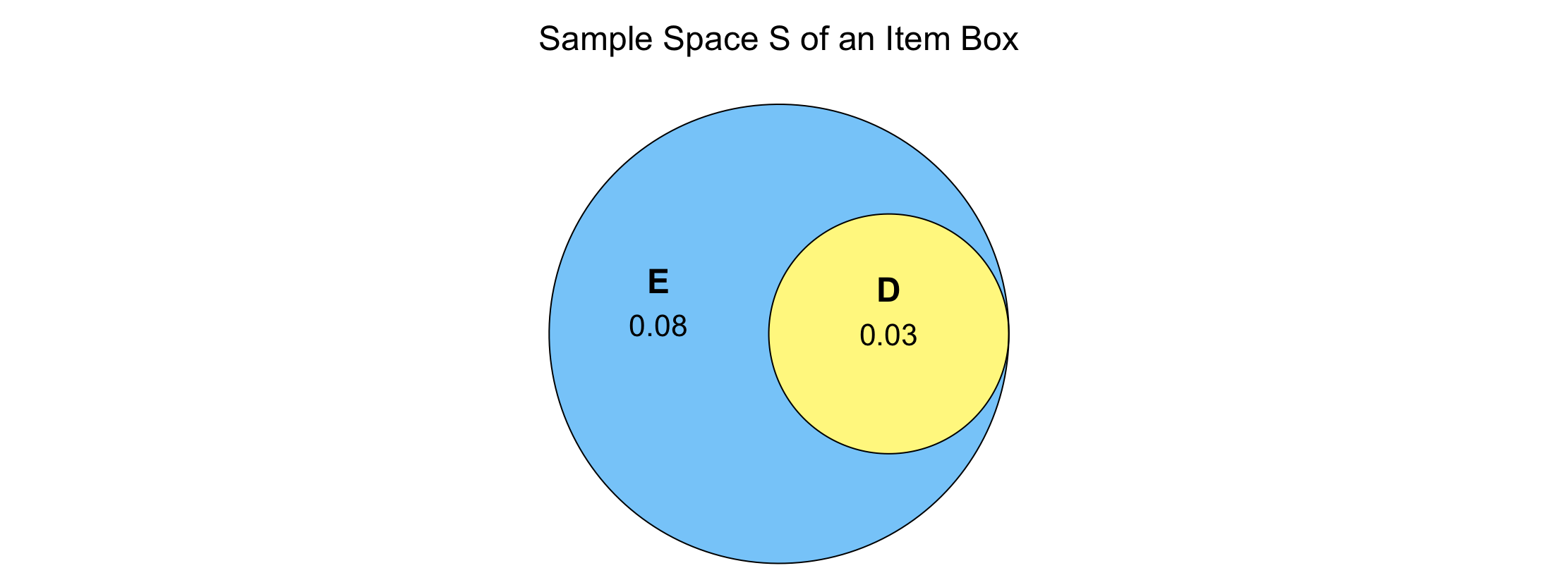
Mutually Exclusive (or Disjoint) Events
- Two events are mutually exclusive (or disjoint) if they cannot happen at the same time in the sample space \(S\):
\[
P(A \cup B) = P(A) + P(B) - \underbrace{P(A \cap B)}_{0} = P(A) + P(B).
\]
Then…
- What is the probability of getting an item that is both an explosion item (event \(E\)) and defeats blue shells (event \(D\))?
Finally…
- What is the probability of getting an item that is an explosion item (event \(E\)) or an item that defeats blue shells (event \(D\))?
Independent Events
- Two events are independent if the occurrence of one of them does not affect the probability of the other.
- Their intersection is defined as: \[P(A \cap B) = P(A) \cdot P(B).\]
1.3. Comparing Probabilities
- We might be interested in comparing two probabilities.
- Suppose an event has a probability \(p\) of happening.
The Odds
- The odds \(o\) are defined as the ratio of this probability to the probability of not happening \(1 - p\): \[o = \frac{p}{1 - p}.\]
- With some algebraic rearrangements, we can obtain \(p\) with the odds: \[p = \frac{o}{o+1}.\]
Example
- If you win 80% of the times at solitaire, i.e., \(p = 0.8\); then your odds are: \[o = \frac{p}{1 - p} = \frac{0.8}{0.2} = 4\]
- This is sometimes written as 4:1 odds – that is, four wins for every loss.
2. Probability Distributions
- A probability distribution is the set of all outcomes and their corresponding probabilities.
- The outcome itself, which is uncertain, is called a random variable; e.g., \[X = \text{Number of customers standing in line at a bank branch.}\]
Types of Random Variables
In general, random variables are classified as:
- Continuous: it can take on a set of uncountable outcomes.
- Discrete: it can take on a set of countable outcomes.
Heads-up: A continuous random variable has a probability density function (PDF), whereas a discrete has a probability mass function (PMF).
Example of a Discrete and Categorical Random Variable
\[Y = \text{Item obtained from the box.}\]
Example of a Discrete and Count Random Variable
\[C = \text{Length of ship stay in days.}\]
| 1 |
0.25 |
| 2 |
0.50 |
| 3 |
0.15 |
| 4 |
0.10 |
3. Measures of Central Tendency and Uncertainty
- These measures summarize the information of a probability distribution.
- They are subset as:
- Central tendency: a “typical” value in a random variable.
- Uncertainty: a measure of how “spread” the random variable is.
3.1. Mode and Entropy in Discrete Random Variables
- Both measures apply to all classes of discrete random variables.
- The mode is a measure of central tendency. It is the outcome having the highest probability.
The Entropy
- It is a measure of uncertainty defined as
\[H(Y) = -\displaystyle \sum_y P(Y = y)\log[P(Y = y)].\]
- It is a nonnegative measure of uncertainty.
- If its value is equal to zero, then there is no randomness.
Example
- What is the mode for \(Y = \text{Item obtained from the box}\)?
How About the Entropy?
\[\begin{align*}
H(Y) &= -\displaystyle \sum_y P(Y = y)\log[P(Y = y)] \\
&= -[0.12 \log(0.12) + 0.05 \log(0.05) + \\
& \qquad \quad 0.75 \log(0.75) + 0.03 \log(0.03) + 0.05 \log(0.05)] \\
&= 0.87
\end{align*}\]
3.2. Mean and Variance
- Both measures apply to both discrete and continuous random variables (as long as they are numeric!).
The Mean
- It is a measure of central tendency.
- If \(X\) is discrete, with \(P(X = x)\) as a PMF, then \[\mathbb{E}(X) = \displaystyle \sum_x x \cdot P(X = x).\]
- If \(X\) is continuous, with \(f_X(x)\) as a PDF, then \[\mathbb{E}(X) = \displaystyle \int_x x \cdot f_X(x) \text{d}x.\]
The Variance
- It is a measure of uncertainty.
\[\text{Var}(X) = \mathbb{E}\{[X - \mathbb{E}(X)]^2\} = \mathbb{E}(X^2) - [\mathbb{E}(X)]^2.\]
- Note it is an expectation (specifically, the squared deviation from the mean).