Parametric Families

Lecture 2

Please, sign in on iClicker

Today’s Learning Goals

By the end of this lecture, we will be able to…

• Calculate expectations of a linear combination of random variables.
• Match a physical process to a distribution family (Binomial, Geometric, Negative Binomial, Poisson, and Bernoulli).
• Calculate probabilities, mean, and variance of a distribution belonging to a distribution family.

And…

• Find the probability mass function of a random variable transformation, e.g., \(X^2\).
• Distinguish between a family of distributions and a distribution.
• Identify whether a specification of parameters (such as mean and variance) is enough/too little/too much to specify a distribution from a family of distributions.

Outline

1. Properties of Distributions
2. Random Variable Transformations
3. Distribution Families
4. Another Common Discrete Distribution Families

1. Properties of Distributions

• We must start getting familiar with central tendency and uncertainty measures from lecture1.
• Hence, let us practice their computations with some in-class iClicker.

1.1. A Single Probability Mass Function

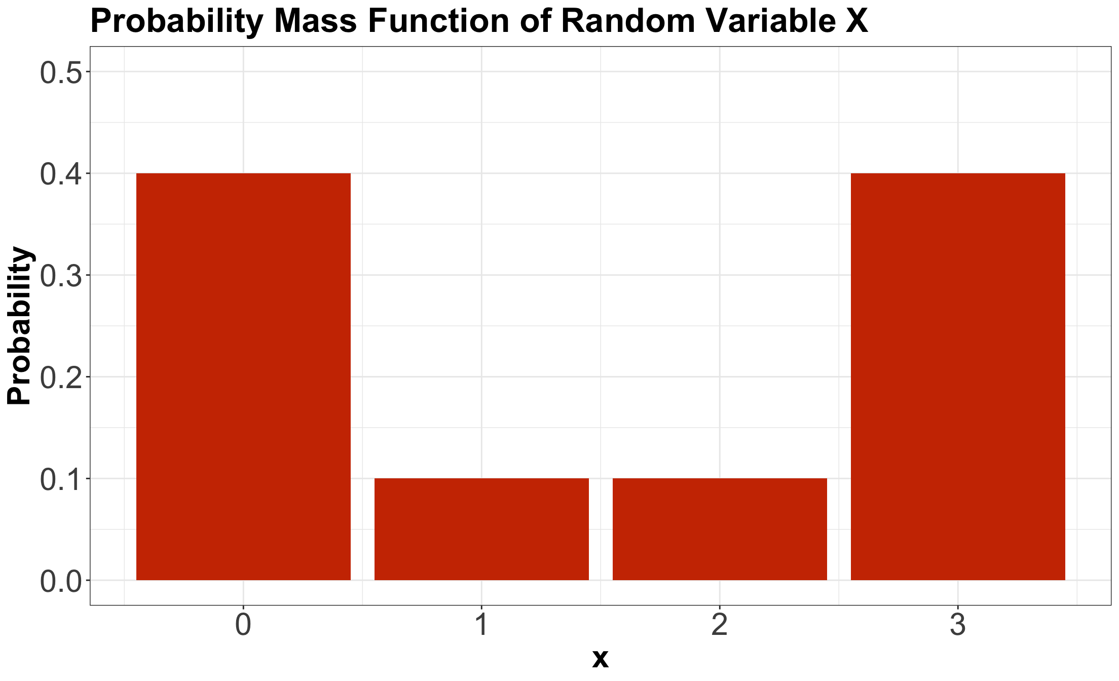
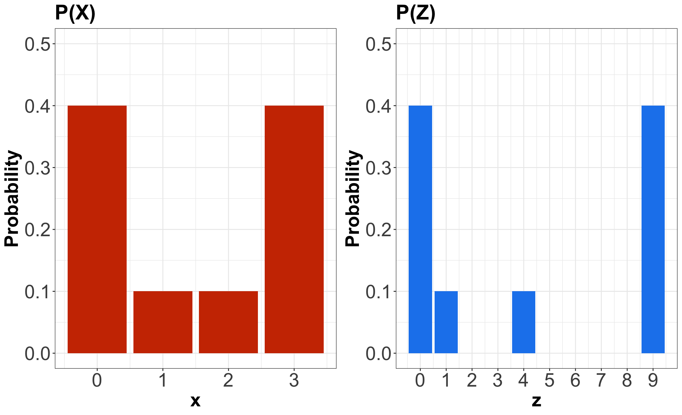
• Suppose \(X\) is a discrete random variable denoting the following: \[X = \text{Number of crabs found at a nest in a Mexican beach.}\]

Probability Mass Function (PMF)

\(X\)	\(P(X = x)\)
0	0.4
1	0.1
2	0.1
3	0.4

We plot it as a bar chart…

iClicker Question

Using the PMF for random variable \(X\), compute \(\mathbb{E}(X)\). Select the correct option:

A. 1

B. 1.5

C. 1.9

D. 6

iClicker Question

Using the PMF for random variable \(X\), compute the variance \(\text{Var}(X)\). Select the correct option:

A. 2.6

B. 1.85

C. 4.1

D. -1.85

iClicker Question

Using the PMF for random variable \(X\), obtain the mode \(\text{Mode}(X)\). Select the correct option:

A. 0

B. 3

C. Both 0 and 3

D. Neither

iClicker Question

Using the PMF for random variable \(X\), obtain the entropy \(H(X).\) Select the correct option:

A. -1.19

B. 0.52

C. -0.52

D. 1.19

1.2. Comparing Multiple Probability Mass Functions

Suppose there are four different random variables related to four Mexican beaches:

\[\begin{gather*} U = \text{Number of crabs found at a nest at Acapulco} \\ V = \text{Number of crabs found at a nest at Cabo San Lucas} \\ W = \text{Number of crabs found at a nest at Cancún} \\ Y = \text{Number of crabs found at a nest at Puerto Vallarta.} \end{gather*}\]

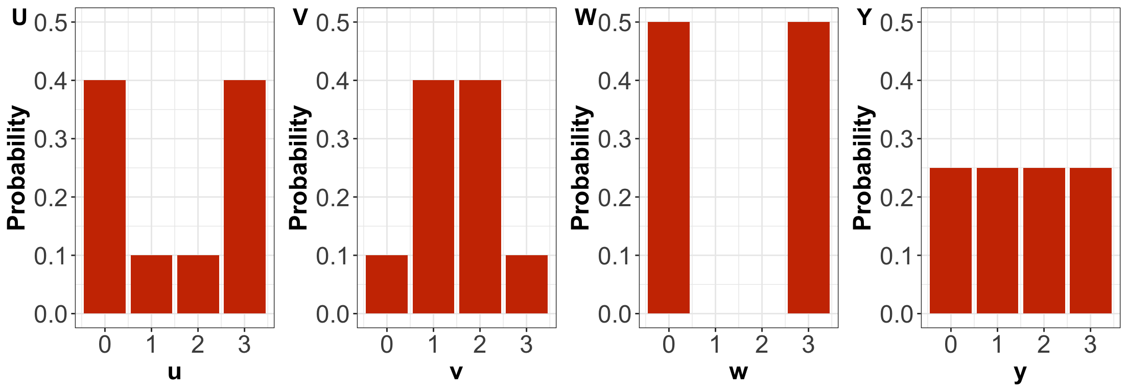
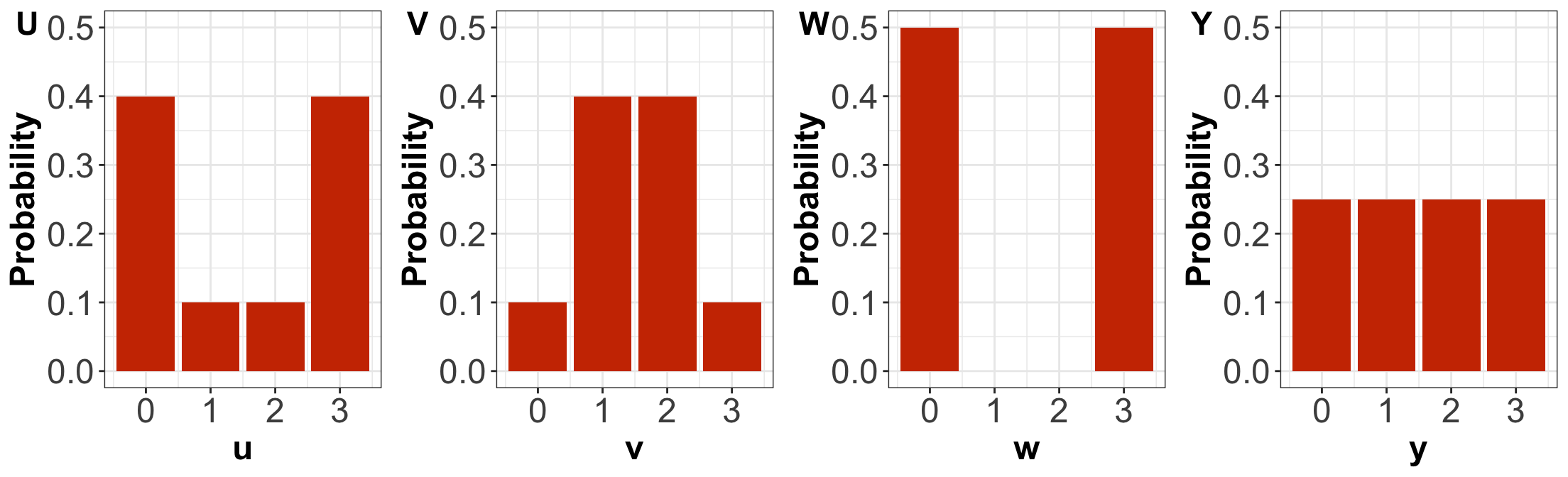
Probability Mass Functions (PMFs)

iClicker Question

Answer TRUE or FALSE:

By only looking at the PMFs, \(U\) has higher entropy than \(V\).

A. TRUE

B. FALSE

iClicker Question

Answer TRUE or FALSE:

By only looking at the PMFs, \(U\) has higher variance than \(V\).

A. TRUE

B. FALSE

iClicker Question

Answer TRUE or FALSE:

By only looking at the PMFs, \(W\) has the highest variance amongst the four distributions.

A. TRUE

B. FALSE

iClicker Question

Answer TRUE or FALSE:

By only looking at the PMFs, \(Y\) has the highest entropy amongst the four distributions.

A. TRUE

B. FALSE

2. Random Variable Transformations

• A random variable can be turned into other random variables via mathematical transformations.
• This characteristic is crucial in data modelling!

2.1. Revisiting Variance

• We can compute the variance of a random variable \(X\) in two forms:

  1. \(\text{Var}(X) = \mathbb{E}\{[X - \mathbb{E}(X)]^2\}\), or alternatively
  2. \(\text{Var}(X) = \mathbb{E}(X^2) - [\mathbb{E}(X)]^2\).

Computing the Variance Using Crabs PMF for \(X\)

Method 1

\[\begin{align*} \text{Var}(X) &= \mathbb{E}\{[X - \mathbb{E}(X)]^2\} \\ &= \mathbb{E}[(X - 1.5)^2] \qquad \qquad \text{since } \mathbb{E}(X) = 1.5 \\ &= (-1.5)^2(0.4) + (-0.5)^2(0.1) + (0.5)^2(0.1) + (1.5)^2(0.4) \\ &= 1.85. \end{align*}\]

Now with the other approach…

Method 2

\[\begin{align*} \text{Var}(X) &= \mathbb{E}(X^2) - [\mathbb{E}(X)]^2 \\ &= \mathbb{E}(X^2) - (1.5)^2 \qquad \qquad \text{since } \mathbb{E}(X) = 1.5 \\ &= (0)^2(0.4) + (1)^2(0.1) + (2)^2(0.1) + (3)^2(0.4) - (1.5)^2 \\ &= 1.85. \end{align*}\]

2.2. Distribution Mapping

• Following up with the crabs PMF, let us focus the attention on \(\mathbb{E}(X^2)\).
• More specifically, what does \(X^2\) mean?
• It comes down to what we define in Statistics as a random variable transformation.
• We can rename \(X^2\) as \[Z = X^2.\]

Comparing PMFs

2.3. Expected Value Properties

• Expected values have certain useful properties.
• If \(a\) and \(b\) are constants, with \(X\) and \(Y\) as random variables, then we can obtain the expected value of the following expressions as:

\[\begin{gather*} \mathbb{E}(a X) = a \mathbb{E}(X) \\ \mathbb{E}(X + Y) = \mathbb{E}(X) + \mathbb{E}(Y) \\ \mathbb{E}(aX + bY) = a\mathbb{E}(X) + b\mathbb{E}(Y). \end{gather*}\]

Caution

• The operator \(\mathbb{E}(\cdot)\) does not follow the usual algebraic rules.
• For instance, if no further assumptions are made for random variables \(X\) and \(Y\), then \[\mathbb{E}(XY) \neq \mathbb{E}(X)\mathbb{E}(Y).\]
• Moreover, note the following: \[\mathbb{E}(X^2) \neq [\mathbb{E}(X)]^2.\]

2.3. Variance Properties

• If \(a\) and \(b\) are constants, with \(X\) and \(Y\) as independent random variables, then we can obtain the variance of the following expressions as:

\[\begin{gather*} \text{Var}(a X) = a^2 \text{Var}(X) \\ \text{Var}(X + Y) = \text{Var}(X) + \text{Var}(Y) \\ \text{Var}(aX + bY) = a^2 \text{Var}(X) + b^2 \text{Var}(Y). \end{gather*}\]

3. Distribution of Families

• A huge component of Data Science is to model data as random variables with uncertain outcomes.
• For instance:
  • The number of ships that arrive at the port of Vancouver on a given day (i.e., a discrete and count random variable).
  • A rock class (i.e., a discrete and categorical random variable).

3.1. Bernoulli

• Suppose you play a game and win with probability \(0 \leq p \leq 1\).
• Let \(X\) be the outcome of this game. It is a binary random variable as follows \[ X = \begin{cases} 1 \; \; \; \; \text{if you win the game (success)},\\ 0 \; \; \; \; \mbox{otherwise}. \end{cases} \]
• The value \(1\) has a probability of \(p\), whereas the value \(0\) has a probability of \(1 - p\).

PMF

• A Bernoulli distribution is depicted as: \[X \sim \text{Bernoulli}(p).\]
• Its PMF is \[P(X = x \mid p) = p^x (1 - p)^{1 - x} \quad \text{for} \quad x = 0, 1.\]

Mean

\[\begin{align*} \mathbb{E}(X) &= \sum_{x = 0}^1 x \cdot P(X = x \mid p) \\ &= \sum_{x = 0}^1 x \cdot p^x (1 - p)^{1 - x} \\ &= p. \end{align*}\]

Variance

\[\begin{align*} \text{Var}(X) &= \mathbb{E}(X^2) - [\mathbb{E}(X)]^2 \\ &= \mathbb{E}(X^2) - p^2 \qquad \qquad \text{since } \mathbb{E}(X) = p \\ &= \sum_{x = 0}^1 x^2 \cdot P(X = x \mid p) - p^2 \\ &= p(1 - p). \end{align*}\]

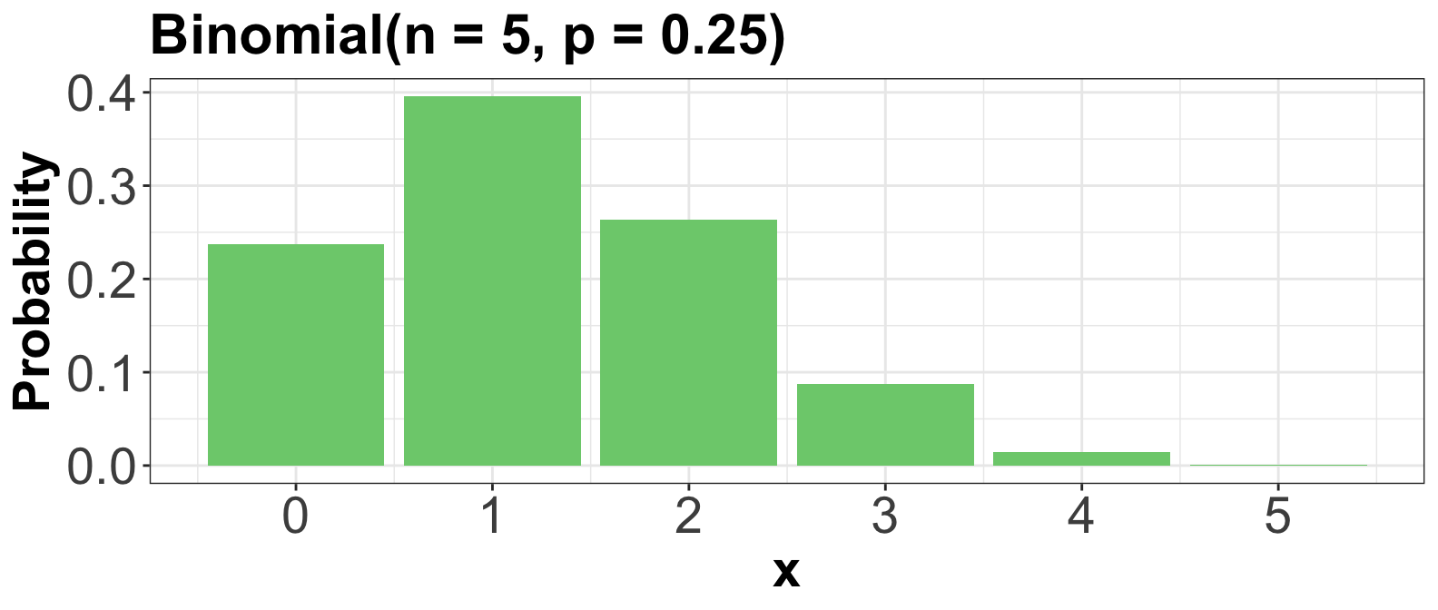
3.2. Binomial

• Suppose you play a game, and win with probability \(0 \leq p \leq 1\).
• Let \(X\) be the number of games you win within \(n\) independent games in total.
• \(X\) is said to have a Binomial distribution, written as \[X \sim \text{Binomial} (n, p).\]

PMF

• A Binomial distribution is characterized by the PMF \[P \left( X = x \mid n, p \right) = {n \choose x} p^x (1 - p)^{n - x} \quad \text{for} \quad x = 0, 1, \dots, n.\]
• The above PMF has the following component: \[{n \choose x} = \frac{n!}{x!(n - x)!}.\]

Example

• Let us derive the probability of winning exactly two games out of five.
• I.e., \(P(X = 2)\) when \(n = 5\) and \(p = 0.25\): \[\begin{align*} P(X = 2 \mid n = 5, p = 0.25) &= {5 \choose 2} (0.25)^2 (1 - 0.25)^{5 - 2} \\ &= \frac{5!}{2!(5 - 2)!} (0.25)^2 (1 - 0.25)^{5 - 2} \\ &= 0.26. \end{align*}\]

Mean and Variance

\[\mathbb{E}(X) = n p\]

\[\text{Var}(X) = n p (1 - p).\]

3.3. Families Versus Distributions

• Specifying a value for both \(p\) and \(n\) results in a unique Binomial distribution.

• There are, in fact, infinite Binomial distributions.

3.4. Parameters

• Since \(p\) and \(n\) fully specify a Binomial distribution, we call them parameters of the Binomial family.
• We call the Binomial family a parametric family of distributions.

3.5. Parameterization

• Which variables we decide to use to identify a distribution within a family is called the family’s parameterization.
• Parameterization will depend on the information you can more easily obtain.

4. Another Common Discrete Distribution Families

• Aside from the Binomial family of distributions, many other families come up in data modelling.
• In practice, distribution families still act as useful approximations.

4.1. Geometric

• Suppose you play a game, and win with probability \(0 \leq p \leq 1\).
• Let \(X\) be the number of independent failures before the first independent success.
• \(X\) is said to have a Geometric distribution, written as \[X \sim \text{Geometric} (p).\]

PMF

• A Geometric distribution is characterized by the PMF \[P(X = x \mid p) = p (1 - p)^x \quad \text{for} \quad x = 0, 1, \dots\]
• Since there is only one parameter, this means that if you know the mean, you also know the variance!
• It has an infinite support.

Mean and Variance

\[\mathbb{E}(X) = \frac{1 - p}{p}\]

\[\text{Var}(X) = \frac{1 - p}{p^2}.\]

4.2. Negative Binomial (a.k.a. Pascal)

• Suppose you play a game, and win with probability \(0 \leq p \leq 1\).
• Let \(X\) be the number of independent losses at playing the game before experiencing \(k\) independent wins.
• \(X\) is said to have a Negative Binomial distribution, written as \[X \sim \text{Negative Binomial} (k, p).\]

PMF

• A Negative Binomial distribution is characterized by the PMF \[P(X = x \mid k, p) = {k - 1 + x \choose x} p^k (1 - p)^x \quad \text{for} \quad x = 0, 1, \dots\]
• It has two parameters: \(k\) and \(p\).
• The Geometric family results with \(k = 1\).

Mean and Variance

\[\mathbb{E}(X) = \frac{k(1 - p)}{p}\]

\[\text{Var}(X) = \frac{k(1 - p)}{p^2}.\]

4.3. Poisson

• Suppose customers independently arrive at a store at some average rate \(\lambda\).
• Then, the total number \(X\) of customers arriving after a pre-specified length of time follows a Poisson distribution: \[X \sim \text{Poisson} (\lambda).\]

PMF

• We can find other examples that are indicative of a Poisson process:
  • The number of ships arriving at Vancouver port on a given day.
  • The number of emails you receive on a given day.
• A Poisson distribution is characterized by the PMF \[P(X = x \mid \lambda) = \frac{\lambda^x \exp(-\lambda)}{x!} \quad \text{for} \quad x = 0, 1, \dots\]

Mean and Variance

\[\mathbb{E}(X) = \lambda\]

\[\text{Var}(X) = \lambda.\]

• A notable property of this family is that the mean is equal to the variance!

4.5. Finally, let us check this mindmap…