Joint Probability

Lecture 3

Please, sign in on iClicker

Today’s Learning Goals

By the end of this lecture, we will be able to…

  • Calculate marginal distributions from a joint distribution of random variables.
  • Describe the probabilistic consequences of working with independent random variables.

And…

  • Calculate and describe covariance in multivariate cases (i.e., with more than one random variable).
  • Calculate and describe two mainstream correlation metrics: Pearson’s correlation and Kendall’s \(\tau_K\).

Outline

  1. Joint Distributions
  2. Independence and Dependence Concepts

1. Joint Distributions


  • So far, we have only considered one random variable at a time which has an univariate distribution.
  • However, we very often have more than one random variable.

Coins come again!

  • Consider two independent fair coins (i.e., two independent Bernoulli random variables!).
  • The sample space is: \(\texttt{HH}\), \(\texttt{HT}\), \(\texttt{TH}\), \(\texttt{TT}\), each with a probability \(0.25\).
  • The joint distribution of this process is the following:
\(X/Y\) \(\texttt{H}\) \(\texttt{T}\)
\(\texttt{H}\) 0.25 0.25
\(\texttt{T}\) 0.25 0.25

Random Variable Setup


  • Let us set the following binary random variables (since each one could only have two outcomes, \(\texttt{H}\) or \(\texttt{T}\)):

\[\begin{gather*} X = \text{First coin's outcome.} \\ Y = \text{Second coin's outcome.} \end{gather*}\]

Computing Probabilities


  • Each cell of the previous joint distribution is computed as:

\[\begin{align*} P(X = \texttt{H} \cap Y = \texttt{H}) &= P(X = \texttt{H}) \cdot P(Y = \texttt{H}) \qquad \text{independence} \\ &= 0.5 \cdot 0.5 \qquad \text{fair coins} \\ &= 0.25. \end{align*}\]

Can we have an univariate setup?

  • Alternatively, we can define the following random variable:

\[Z = \text{Outcomes obtained when tossing two independent coins.}\]

Outcome Probability
\(\texttt{HH}\) 0.25
\(\texttt{HT}\) 0.25
\(\texttt{TH}\) 0.25
\(\texttt{TT}\) 0.25

1.1. Example: Length of Stay Versus Gang Demand

  • We will work with the following joint distribution of length of stay (\(\text{LOS}\)) of a ship and its gang demand (\(\text{Gangs}\)).
  • Consider an example that a Vancouver port faces with gang demand.
  • When a ship arrives, they request a certain number of gangs to unload the ship.

Probability Mass Function (PMF) for Gangs

PMF for Length of Stay

LOS Probability
1 0.25
2 0.35
3 0.20
4 0.10
5 0.10

Now, we might wonder…


What is the probability that a ship requires 4 gangs AND will stay in port for 5 days?

  • The information provided by both separate PMFs (\(\text{Gangs}\) and \(\text{LOS}\)) is not sufficient to answer this question.
  • We would need to use a joint distribution between \(\text{LOS}\) and \(\text{Gangs}\).

Before, let us define the following:

  • In a random system/process with more than one random variable, the distribution of a standalone variable is called a marginal distribution.

Now, going back to the joint distribution…

  • We need a probability for every possible combination of the number of \(\text{Gangs}\) and \(\text{LOS}\).
  • In this case, \(5 \times 4 = 20\) probabilities (that again add up to 1).
Gangs = 1 Gangs = 2 Gangs = 3 Gangs = 4
LOS = 1 0.00170 0.04253 0.12471 0.08106
LOS = 2 0.02664 0.16981 0.13598 0.01757
LOS = 3 0.05109 0.11563 0.03203 0.00125
LOS = 4 0.04653 0.04744 0.00593 0.00010
LOS = 5 0.07404 0.02459 0.00135 0.00002

Now, we might wonder…


Could the 20 numbers in the joint distribution be absolutely ANY probabilities between 0 and 1?

  • No, we have the following restrictions:

    • They are restricted by the fact that they will need to add up to 1 (recall the Law of Total Probability!).
    • We need the joint distribution to be consistent with those marginal distributions.

1.2. Calculating Marginal Distributions from the Joint Distribution

  • In the case of discrete random variables, we add up the probabilities of the corresponding standalone outcomes.
Gangs = 1 Gangs = 2 Gangs = 3 Gangs = 4
LOS = 1 0.00170 0.04253 0.12471 0.08106
LOS = 2 0.02664 0.16981 0.13598 0.01757
LOS = 3 0.05109 0.11563 0.03203 0.00125
LOS = 4 0.04653 0.04744 0.00593 0.00010
LOS = 5 0.07404 0.02459 0.00135 0.00002

Let us start with the marginal distribution of \(\text{LOS}\)


  • We can compute \(P(\text{LOS} = 1)\).
  • Thus, there are four ways this could happen:
    • \(\text{LOS} = 1\) and \(\text{Gangs} = 1\).
    • \(\text{LOS} = 1\) and \(\text{Gangs} = 2\).
    • \(\text{LOS} = 1\) and \(\text{Gangs} = 3\).
    • \(\text{LOS} = 1\) and \(\text{Gangs} = 4\).

So, to find the marginal probability \(P(\text{LOS} = 1)\)


\[\begin{align*} P(\text{LOS} = 1) &= P(\text{LOS} = 1 \cap \text{Gangs} = 1) + \\ & \quad \quad P(\text{LOS} = 1 \cap \text{Gangs} = 2) + \\ & \quad \quad \quad P(\text{LOS} = 1 \cap \text{Gangs} = 3) + \\ & \quad \quad \quad \quad P(\text{LOS} = 1 \cap \text{Gangs} = 4) \\ &= 0.00170 + 0.04253 + 0.12471 + 0.08106 \\ &= 0.25. \end{align*}\]

We have \(P(\text{LOS} = 1)\)

  • But we would also need \(P(\text{LOS} = 2)\), \(P(\text{LOS} = 3)\), etc.
  • Thus, we add up each row from our joint distribution.
rowSums(joint_distribution) |>
  kable(col.names = "Probability", align = "c") |>
  kable_styling(font_size = 30) |>
  column_spec(1, bold = TRUE)
Probability
LOS = 1 0.25
LOS = 2 0.35
LOS = 3 0.20
LOS = 4 0.10
LOS = 5 0.10

Now for \(\text{Gangs}\)!

colSums(joint_distribution) |>
  kable(col.names = "Probability", align = "c") |>
  kable_styling(font_size = 30) |>
  column_spec(1, bold = TRUE)
Probability
Gangs = 1 0.2
Gangs = 2 0.4
Gangs = 3 0.3
Gangs = 4 0.1


  • Note both marginals computed from the joint are consistent with our initial marginals.

iClicker Question


Answer TRUE or FALSE:


We obtain a marginal distribution by summing the rows of a joint distribution; therefore, each row of a joint distribution must sum to 1.

A. TRUE

B. FALSE

2. Independence and Dependence Concepts

  • A big part of Data Science is about harvesting the relationship between the variables in our datasets.


2.1. Independence


  • Let \(X\) and \(Y\) be two random variables.
  • \(X\) and \(Y\) are independent if knowing something about one of them tells us nothing about the other: \[P(X = x \cap Y = y) = P(X = x) \cdot P(Y = y).\]
  • We would only need the marginals to obtain their joint distribution.

Going back to the two coins!

  • Recall we had this joint distribution:

\[\begin{gather*} X = \text{First coin's outcome.} \\ Y = \text{Second coin's outcome.} \end{gather*}\]

\(X/Y\) \(\texttt{H}\) \(\texttt{T}\)
\(\texttt{H}\) 0.25 0.25
\(\texttt{T}\) 0.25 0.25

Obtaining the Marginals from the Joint

We can see that the two coin flips are independent:

\[\begin{align*} P(X = \texttt{H}) &= P(X = \texttt{H} \cap Y = \texttt{H}) + P(X = \texttt{H} \cap Y = \texttt{T}) \\ &= 0.25 + 0.25 = 0.5 \\ P(X = \texttt{T}) &= P(X = \texttt{T} \cap Y = \texttt{H}) + P(X = \texttt{T} \cap Y = \texttt{T}) \\ &= 0.25 + 0.25 = 0.5 \\ P(Y = \texttt{H}) &= P(X = \texttt{H} \cap Y = \texttt{H}) + P(X = \texttt{T} \cap Y = \texttt{H}) \\ &= 0.25 + 0.25 = 0.5 \\ P(Y = \texttt{T}) &= P(X = \texttt{H} \cap Y = \texttt{T}) + P(X = \texttt{T} \cap Y = \texttt{T}) \\ &= 0.25 + 0.25 = 0.5. \end{align*}\]

Applying the Independence Property via the Marginals


\[\begin{align*} P(X = \texttt{H} \cap Y = \texttt{H}) &= P(X = \texttt{H}) \cdot P(Y = \texttt{H}) \\ &= 0.5 \cdot 0.5 = 0.25 \\ P(X = \texttt{H} \cap Y = \texttt{T}) &= P(X = \texttt{H}) \cdot P(Y = \texttt{T}) \\ &= 0.5 \cdot 0.5 = 0.25 \\ P(X = \texttt{T} \cap Y = \texttt{H}) &= P(X = \texttt{T}) \cdot P(Y = \texttt{H}) \\ &= 0.5 \cdot 0.5 = 0.25 \\ P(X = \texttt{T} \cap Y = \texttt{T}) &= P(X = \texttt{T}) \cdot P(Y = \texttt{T}) \\ &= 0.5 \cdot 0.5 = 0.25. \end{align*}\]

Let us check another two-coin case…

\[\begin{gather*} X = \text{First coin's outcome} \\ Y = \text{Second coin's outcome.} \end{gather*}\]

\(X/Y\) \(\texttt{H}\) \(\texttt{T}\)
\(\texttt{H}\) 0.2 0.6
\(\texttt{T}\) 0.05 0.15


Computing the Marginals


\[\begin{align*} P(X = \texttt{H}) &= P(X = \texttt{H} \cap Y = \texttt{H}) + P(X = \texttt{H} \cap Y = \texttt{T}) \\ &= 0.2 + 0.6 \\ &= 0.8. \end{align*}\]

  • By the Law of Total Probability, we can obtain: \[\begin{align*} P(X = \texttt{T}) &= 1 - P(X = \texttt{H})\\ &= 1 - 0.8 \\ &= 0.2. \end{align*}\]

And likewise for the second coin…


\[\begin{align*} P(Y = \texttt{H}) &= P(X = \texttt{H} \cap Y = \texttt{H}) + P(X = \texttt{T} \cap Y = \texttt{H}) \\ &= 0.2 + 0.05 \\ &= 0.25. \end{align*}\]

  • By the Law of Total Probability, we can obtain: \[\begin{align*} P(Y = \texttt{T}) &= 1 - P(Y = \texttt{H})\\ &= 1 - 0.25 \\ &= 0.75. \end{align*}\]

Applying the Independence Property via the Marginals

  • These two coins are also independent!

\[\begin{align*} P(X = \texttt{H} \cap Y = \texttt{H}) &= P(X = \texttt{H}) \cdot P(Y = \texttt{H}) \\ &= 0.8 \cdot 0.25 = 0.2 \\ P(X = \texttt{H} \cap Y = \texttt{T}) &= P(X = \texttt{H}) \cdot P(Y = \texttt{T}) \\ &= 0.8 \cdot 0.75 = 0.6 \\ P(X = \texttt{T} \cap Y = \texttt{H}) &= P(X = \texttt{T}) \cdot P(Y = \texttt{H}) \\ &= 0.2 \cdot 0.25 = 0.05 \\ P(X = \texttt{T} \cap Y = \texttt{T}) &= P(X = \texttt{T}) \cdot P(Y = \texttt{T}) \\ &= 0.2 \cdot 0.75 = 0.15. \end{align*}\]

But there is no independence in this other two-coin case!

\[\begin{gather*} X = \text{First coin's outcome} \\ Y = \text{Second coin's outcome.} \end{gather*}\]

\(X/Y\) \(\texttt{H}\) \(\texttt{T}\)
\(\texttt{H}\) 0.5 0
\(\texttt{T}\) 0 0.5


2.2. Measures of Dependence

  • Let us ask ourselves the following:

What if two random variables are not independent?

Is there some measure of dependence?

2.2.1. Covariance and Pearson’s Correlation


  • Covariance is one common way of measuring dependence between two numeric random variables.
  • It measures the amount of dependence and direction:

\[\begin{align*} \operatorname{Cov}(X, Y) &= \mathbb{E}[(X-\mu_X)(Y-\mu_Y)] \\ &= \mathbb{E}(XY) - \mathbb{E}(X)\mathbb{E}(Y). \end{align*}\]

Going back to our cargo ship example!

joint_distribution |>
  kable(align = "cccc") |>
  kable_styling(font_size = 30) |>
  column_spec(1, bold = TRUE)
Gangs = 1 Gangs = 2 Gangs = 3 Gangs = 4
LOS = 1 0.00170 0.04253 0.12471 0.08106
LOS = 2 0.02664 0.16981 0.13598 0.01757
LOS = 3 0.05109 0.11563 0.03203 0.00125
LOS = 4 0.04653 0.04744 0.00593 0.00010
LOS = 5 0.07404 0.02459 0.00135 0.00002
  • For a larger \(\text{LOS}\), there are larger probabilities associated with a smaller gang demand.

Coding Up the Marginal PMFs

Marginal_PMF_LOS <- tribble(
  ~n_days, ~p,
  1, 0.25,
  2, 0.35,
  3, 0.2,
  4, 0.1,
  5, 0.1
)
Marginal_PMF_LOS

Marginal_PMF_Gangs <- tribble(
  ~n_gangs, ~p,
  1, 0.2,
  2, 0.4,
  3, 0.3,
  4, 0.1,
)
Marginal_PMF_Gangs
# A tibble: 5 × 2
  n_days     p
   <dbl> <dbl>
1      1  0.25
2      2  0.35
3      3  0.2 
4      4  0.1 
5      5  0.1 
# A tibble: 4 × 2
  n_gangs     p
    <dbl> <dbl>
1       1   0.2
2       2   0.4
3       3   0.3
4       4   0.1

Computing Marginals Expected Values

E_LOS <- sum(Marginal_PMF_LOS$n_days * Marginal_PMF_LOS$p)
E_LOS

E_Gangs <- sum(Marginal_PMF_Gangs$n_gangs * Marginal_PMF_Gangs$p)
E_Gangs
[1] 2.45
[1] 2.3


Hence:

\[\mathbb{E}(\text{LOS}) = 2.45\] \[\mathbb{E}(\text{Gangs}) = 2.3.\]

Melting joint_distribution (manually!)

joint_distribution <- data.frame(
  LOS = c(rep(1, 4), rep(2, 4), rep(3, 4), rep(4, 4), rep(5, 4)),
  Gangs = rep(1:4, 5),
  p = c(
    0.00170, 0.04253, 0.12471, 0.08106,
    0.02664, 0.16981, 0.13598, 0.01757,
    0.05109, 0.11563, 0.03203, 0.00125,
    0.04653, 0.04744, 0.00593, 0.00010,
    0.07404, 0.02459, 0.00135, 0.00002
  )
)
joint_distribution
   LOS Gangs       p
1    1     1 0.00170
2    1     2 0.04253
3    1     3 0.12471
4    1     4 0.08106
5    2     1 0.02664
6    2     2 0.16981
7    2     3 0.13598
8    2     4 0.01757
9    3     1 0.05109
10   3     2 0.11563
11   3     3 0.03203
12   3     4 0.00125
13   4     1 0.04653
14   4     2 0.04744
15   4     3 0.00593
16   4     4 0.00010
17   5     1 0.07404
18   5     2 0.02459
19   5     3 0.00135
20   5     4 0.00002

Computing the Crossed Expected Value

E_LOS_Gangs <- sum(joint_distribution$LOS *
  joint_distribution$Gangs *
  joint_distribution$p)
E_LOS_Gangs
[1] 4.89956


Thus:

\[\mathbb{E}(\text{LOS} \cdot \text{Gangs}) = 4.89956.\]

Computing the Covariance


\[\begin{align*} \operatorname{Cov}(\text{LOS}, \text{Gangs}) &= \mathbb{E}(\text{LOS} \cdot \text{Gangs}) - \mathbb{E}(\text{LOS})\mathbb{E}(\text{Gangs}) \\ &= 4.89956 - \left[ (2.45)(2.3) \right] \\ &= -0.73544. \end{align*}\]

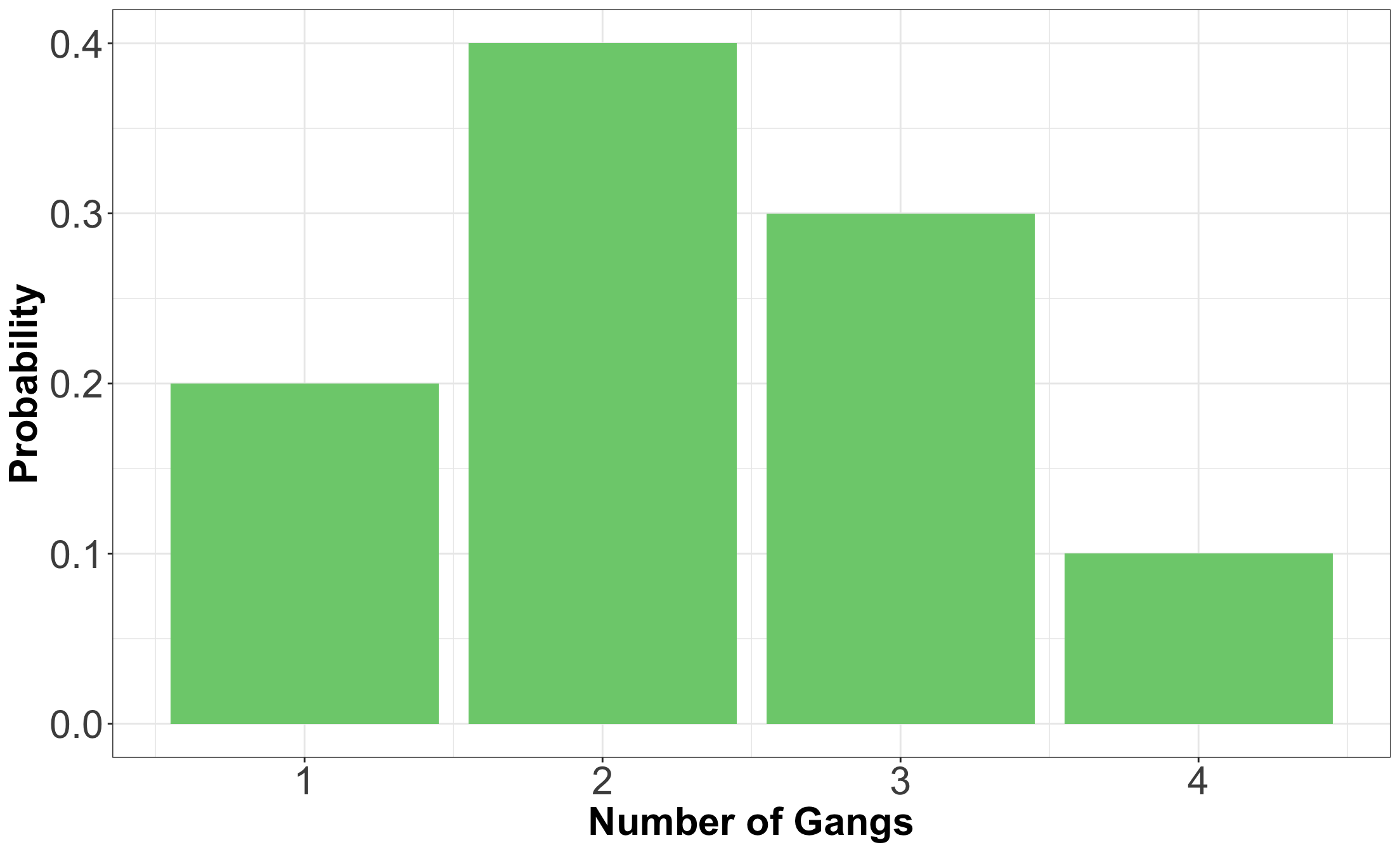
  • Indeed, we can see that the covariance between \(\text{LOS}\) and \(\text{Gangs}\) is negative.
  • A negative sign indicates that an increase in \(\text{LOS}\) is associated with a decrease in \(\text{Gangs}\).

Covariance Drawback

  • This measure depends on the spread of the random variables \(X\) and \(Y\).
  • For instance, if we multiply \(X\) by 10, then the covariance of \(X\) and \(Y\) increases by a factor of 10 as well: \[\begin{align*} \operatorname{Cov}(10X,Y) &= \mathbb{E}(10XY) - \mathbb{E}(10X) \mathbb{E}(Y) \\ &= 10\mathbb{E}(XY) - 10\mathbb{E}(X)\mathbb{E}(Y) \\ &= 10[\mathbb{E}(XY) - \mathbb{E}(X) \mathbb{E}(Y)] \\ &= 10\operatorname{Cov}(X,Y). \end{align*}\]

Pearson’s Correlation

  • Pearson’s correlation standardizes the distances according to the standard deviations \(\sigma_X\) and \(\sigma_Y\) of \(X\) and \(Y\), respectively. \[\begin{align*} \operatorname{Corr}(X, Y) &= \mathbb{E} \left[ \left(\frac{X-\mu_X}{\sigma_X}\right) \left(\frac{Y-\mu_Y}{\sigma_Y}\right) \right] \\ &= \frac{\operatorname{Cov}(X, Y)}{\sqrt{\operatorname{Var}(X)\operatorname{Var}(Y)}}. \end{align*}\]
  • It turns out that \(-1 \leq \text{Corr}(X, Y) \leq 1\).

Pearson’s Correlation Scale


  • \(-1\) means a perfect negative linear relationship between \(X\) and \(Y\).
  • \(0\) means no linear relationship (however, this does not mean independence!).
  • \(1\) means a perfect positive linear relationship.

iClicker Question


Answer TRUE or FALSE:


Covariance can be negative, but not the variance.

A. TRUE

B. FALSE

iClicker Question

Answer TRUE or FALSE:

Without any further assumptions between random variables \(X\) and \(Y\), covariance is calculated as

\[\operatorname{Cov}(X,Y) = \mathbb{E}(XY) - \left[ \mathbb{E}(X) \mathbb{E}(Y) \right].\]

Computing \(\mathbb{E}(XY)\) requires the joint distribution, but computing \(\mathbb{E}(X) \mathbb{E}(Y)\) only requires the marginals.


A. TRUE

B. FALSE

2.2.2. Kendall’s \(\tau_K\)


  • Pearson’s correlation measures linear dependence.
  • This might be a big downfall, since many relationships between real-world variables are not linear.
  • Hence, there is an alternative measure called Kendall’s \(\tau_K\).

Characteristics of Kendall’s \(\tau_K\)

  • Kendall’s \(\tau_K\) can measure non-linear dependence.
  • It measures concordance between each pair of observations \((x_i, y_i)\) and \((x_j, y_j)\) with \(i \neq j\):
Concordant means \[\begin{gather*} x_i < x_j \quad \text{and} \quad y_i < y_j, \\ \text{or} \\ x_i > x_j \quad \text{and} \quad y_i > y_j; \end{gather*}\] which gets a positive sign.

Characteristics of Kendall’s \(\tau_K\)


Discordant means \[\begin{gather*} x_i < x_j \quad \text{and} \quad y_i > y_j, \\ \text{or} \\ x_i > x_j \quad \text{and} \quad y_i < y_j; \end{gather*}\] which gets a negative sign.

Formal Definition

  • Kendall’s \(\tau_K\) averages the amount of concordance and discordance by taking the difference between the number of concordant and number of discordant pairs.
  • The formal definition with \(n\) data pairs is

\[\tau_K = \frac{\text{Number of concordant pairs} - \text{Number of discordant pairs}}{{n \choose 2}}.\]

  • Kendall’s \(\tau_K\) is between -1 and 1, and measures dependence’s strength (and direction).
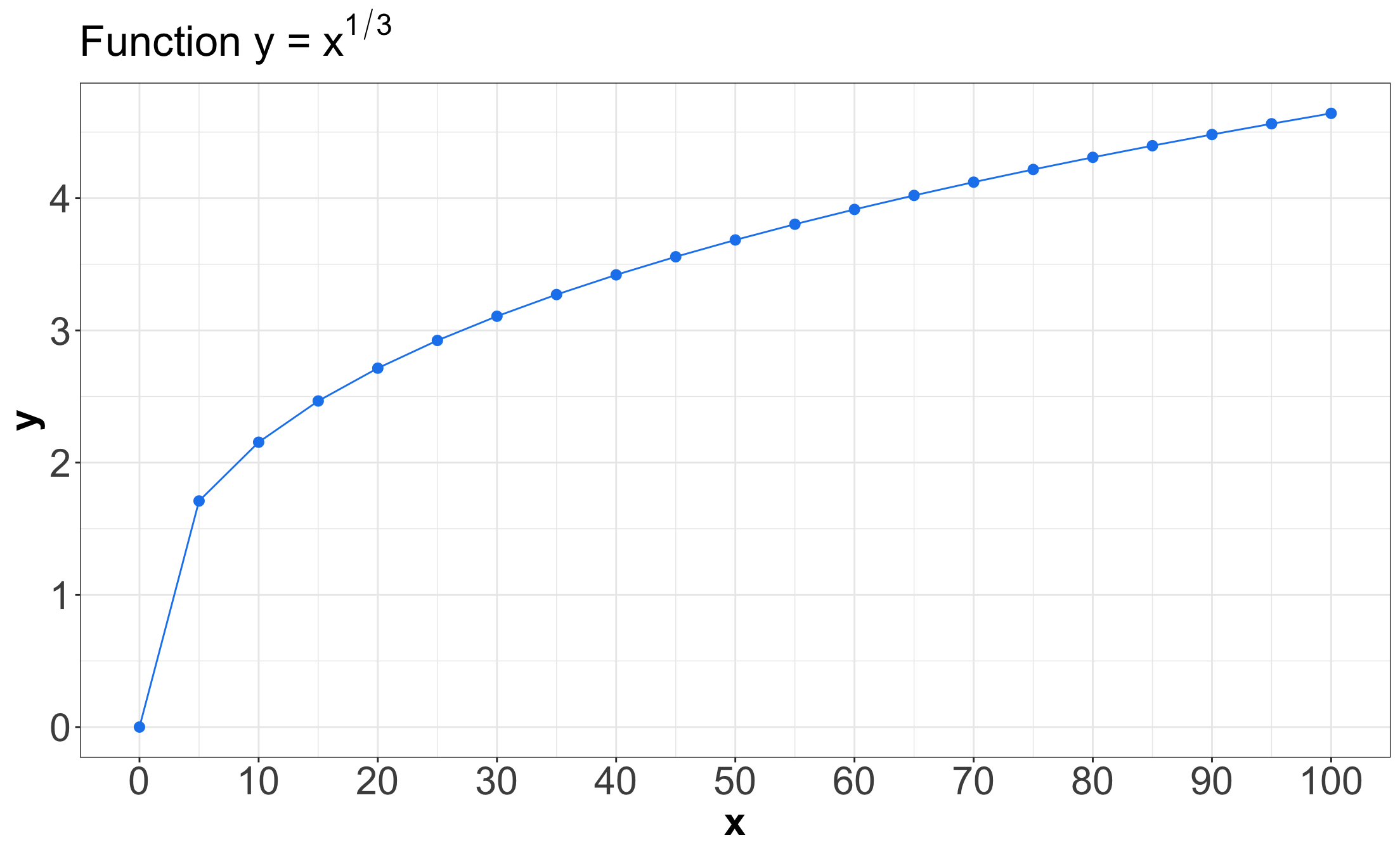
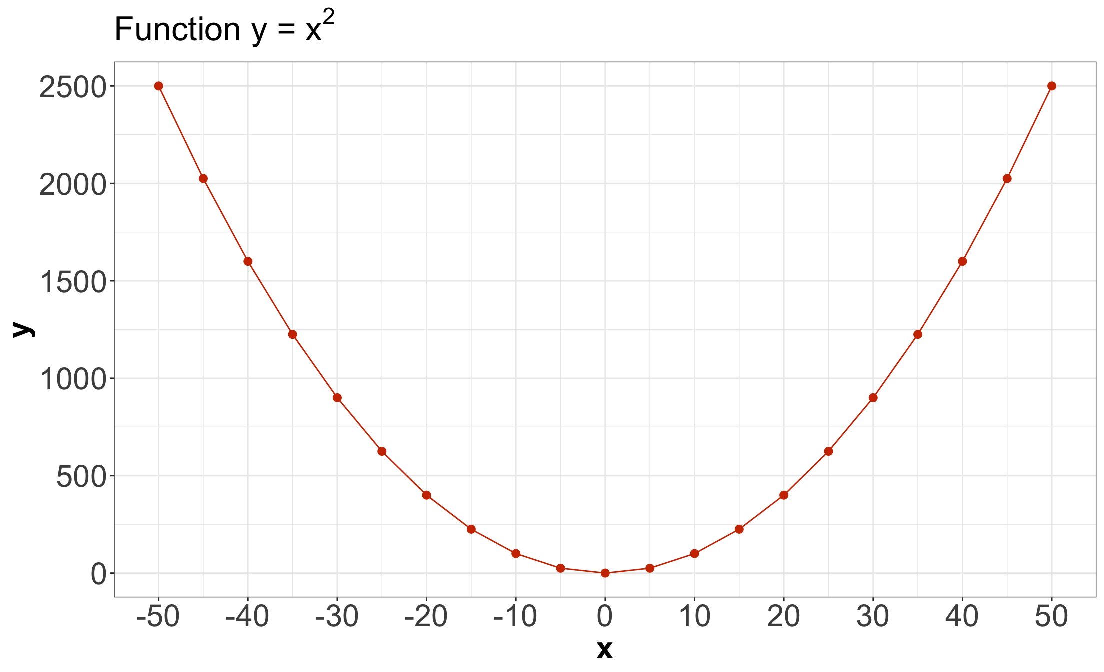
First Example


  • Consider the two correlation measures: Pearson and Kendall’s \(\tau_K\).
  • We will hypothetical dataset called non_linear_function with \(n = 21\) where: \[y = x^{1/3}.\]

Coding Up non_linear_function


non_linear_pairs <- tibble(
  x = seq(from = 0, to = 100, by = 5),
  y = x^(1 / 3)
)
non_linear_pairs
# A tibble: 21 × 2
       x     y
   <dbl> <dbl>
 1     0  0   
 2     5  1.71
 3    10  2.15
 4    15  2.47
 5    20  2.71
 6    25  2.92
 7    30  3.11
 8    35  3.27
 9    40  3.42
10    45  3.56
# ℹ 11 more rows

Plotting non_linear_function

Computing Correlation Metrics


tribble(
  ~Pearson, ~Kendall,
  round(cor(non_linear_pairs, method = "pearson")[1, 2], 4),
  round(cor(non_linear_pairs, method = "kendall")[1, 2], 4)
) |>
  knitr::kable(align = "cc")
Pearson Kendall
0.9097 1

Second Example


  • Consider the two correlation measures: Pearson and Kendall’s \(\tau_K\).
  • We will hypothetical dataset called parabola_pairs with \(n = 21\) where: \[y = x^2.\]

Coding Up parabola_pairs


parabola_pairs <- tibble(
  x = seq(from = -50, to = 50, by = 5),
  y = x^2
)
parabola_pairs
# A tibble: 21 × 2
       x     y
   <dbl> <dbl>
 1   -50  2500
 2   -45  2025
 3   -40  1600
 4   -35  1225
 5   -30   900
 6   -25   625
 7   -20   400
 8   -15   225
 9   -10   100
10    -5    25
# ℹ 11 more rows

Plotting parabola_pairs

Computing Correlation Metrics

tribble(
  ~Pearson, ~Kendall,
  round(cor(parabola_pairs, method = "pearson")[1, 2], 4),
  round(cor(parabola_pairs, method = "kendall")[1, 2], 4)
) |>
  knitr::kable(align = "cc")
Pearson Kendall
0 0


  • Patterns like a parabola are not monotonically increasing or decreasing.
  • Thus, neither Pearson nor Kendall’s \(\tau_K\) will capture the parabola pattern.

2.3. Variance of a Sum Involving Two Non-Independent Random Variables


  • Suppose \(X\) and \(Y\) are not independent random variables.
  • Therefore: \[\operatorname{Var}(X + Y) = \operatorname{Var}(X) + \operatorname{Var}(Y) + 2\operatorname{Cov}(X, Y).\]

If \(X\) and \(Y\) are independent, then…

\[\mathbb{E}(XY) = \mathbb{E}(X) \mathbb{E}(Y).\]

  • Finally:

\[\begin{align*} \operatorname{Var}(X + Y) &= \operatorname{Var}(X) + \operatorname{Var}(Y) + 2\operatorname{Cov}(X, Y) \\ &= \operatorname{Var}(X) + \operatorname{Var}(Y) + 2 \left\{ \mathbb{E}(XY) - \left[ \mathbb{E}(X)\mathbb{E}(Y) \right] \right\} \\ &= \operatorname{Var}(X) + \operatorname{Var}(Y) + 2 \underbrace{\left\{ \left[ \mathbb{E}(X) \mathbb{E}(Y) \right] - \left[ \mathbb{E}(X)\mathbb{E}(Y) \right] \right\}}_{0} \\ &= \operatorname{Var}(X) + \operatorname{Var}(Y). \end{align*}\]