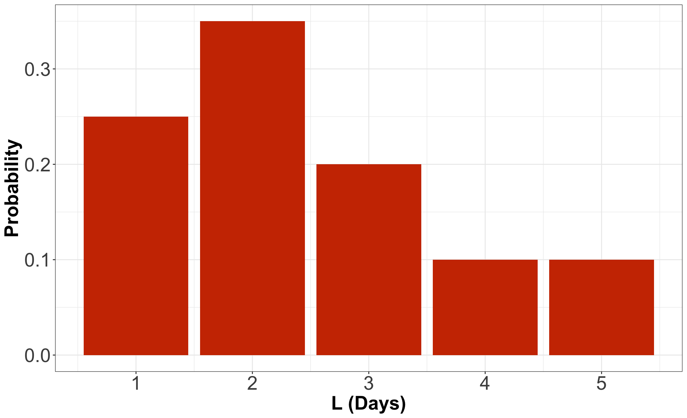
| L (Days) | Probability |
|---|---|
| 1 | 0.25 |
| 2 | 0.35 |
| 3 | 0.20 |
| 4 | 0.10 |
| 5 | 0.10 |
Conditional Probabilities
Lecture 4
1. Univariate Conditional Distributions
Probability distributions describe an uncertain outcome, but what if we have partial information?

Example: Length of Stay Versus Gang Demand
- Consider the example of ships arriving at the port of Vancouver again.
- Each ship will stay at port for a random number of days, which we will call the length of stay (\(\text{LOS}\)).

PMF of Length of Stay as a Bar Chart
Conditional Probability
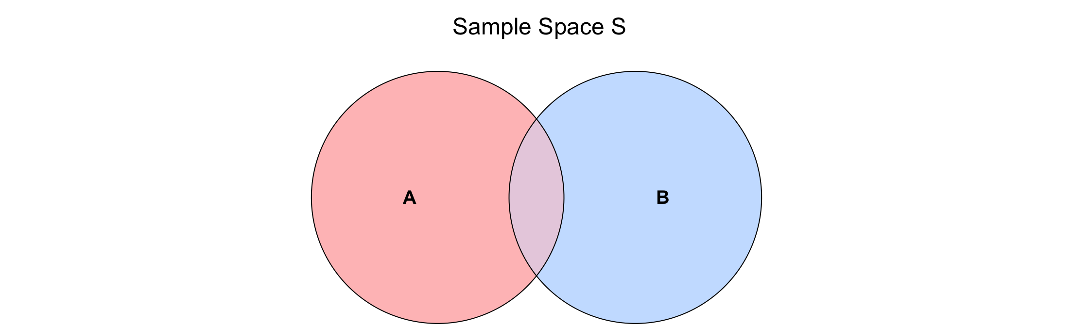
- Let \(A\) and \(B\) be two events of interest within the sample \(S\), and \(P(B) > 0\), then the conditional probability of \(A\) given \(B\) is defined as: \[P(A \mid B) = \frac{P(A \cap B)}{P(B)}.\]
- Event \(B\) is becoming the new sample space (note that \(P(B \mid B) = 1\)).
Graphically…
\[P(A \mid B) = \frac{P(A \cap B)}{P(B)}\]
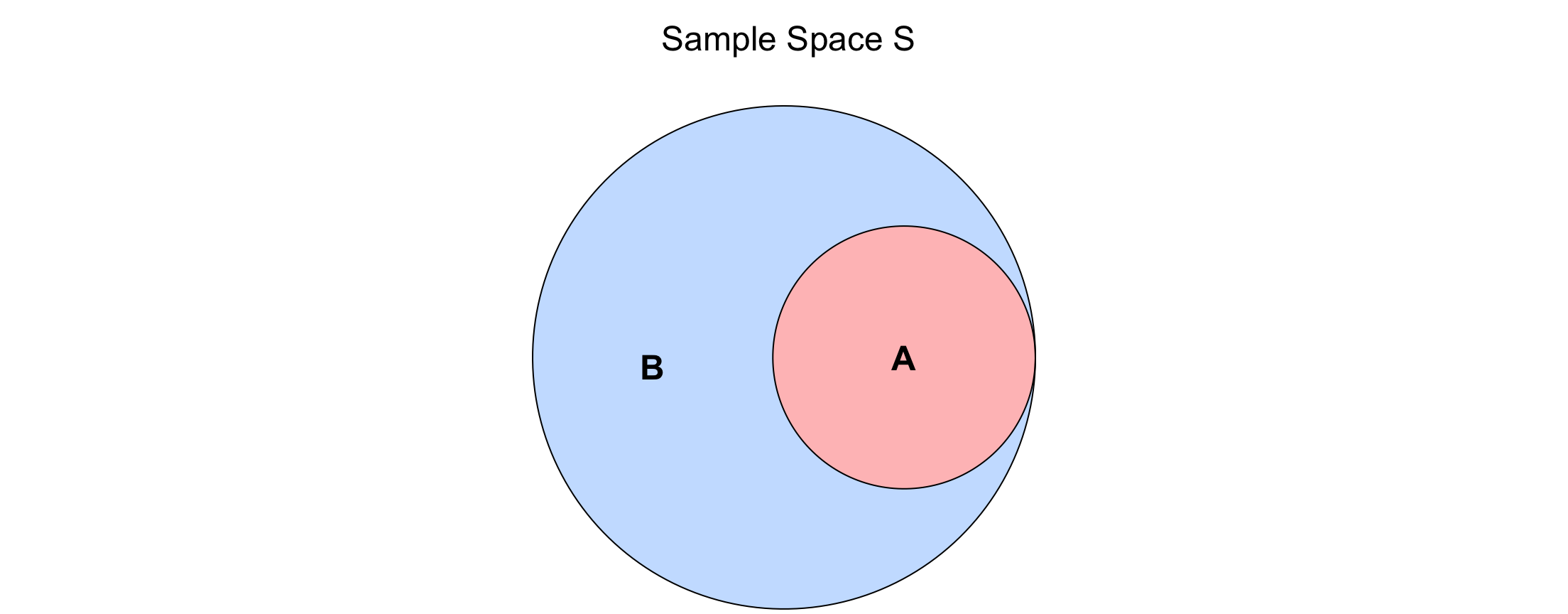
Another depiction…
\[P(A \mid B) = \frac{P(A \cap B)}{P(B)} = \frac{P(A)}{P(B)}\]
Conditional Probability Distribution
- A conditional probability distribution of event \(A\) given \(B\) is a proper probability distribution for event \(A\) after observing event \(B\).
- This distribution is restricted to the subsample space provided by event \(B\).
Goin back to the ships!
- Suppose a ship has been at port for 2 days now, and it will be staying longer. This means that we know that \(L\) will be greater than 2.
- What is the distribution of the \(\text{LOS}\) now? Using symbols, this is written as \[P(L = l \mid L > 2).\]
Applying Conditional Concepts
- \(P(L = 3 \mid L > 2)\), is a conditional probability,
- and the whole distribution, \(P(L = l \mid L > 2)\) for all \(l\), is called a conditional probability distribution.
- Therefore: \[\displaystyle \sum_{l = 3}^5 P(L = l \mid L > 2) = 1.\]
Recall the original PMF in our ship example!
| L (Days) | Probability |
|---|---|
| 1 | 0.25 |
| 2 | 0.35 |
| 3 | 0.20 |
| 4 | 0.10 |
| 5 | 0.10 |
Second Step of Re-normalization
- We scale (or re-normalize) their corresponding probabilities up to bigger values so that they all add up to 1 again.
- In this case,
\[0.20 + 0.10 + 0.10 = 0.40.\]
Re-normalized Table
- If we divide all the probabilities by \(0.4\), we will be good to go:
| L (Days) | Probability |
|---|---|
| 1 | 0 |
| 2 | 0 |
| 3 | 0.50 |
| 4 | 0.25 |
| 5 | 0.25 |
1.2. Formula Approach
- Let us use the conditional probability formula: \[\begin{align*} P(L = l \mid L > 2) &= \frac{P(L = l \cap L > 2)}{P(L > 2)} = \frac{P(L = l)}{P(L > 2)} \\ & \qquad \qquad \qquad\qquad \quad \text{for} \quad l = 3, 4, 5. \end{align*}\]
Checking the Numerator
- How did we reduce the convoluted event \(L = l \cap L > 2\) to the simple event \(L = l\) for \(l = 3, 4, 5\)?
- We go through all outcomes and check which ones satisfy the requirement \[L = l \cap L > 2.\]
- This reduces to \(L = l\), as long as \(l = 3, 4, 5\).
Applying the Formula
- Let us recheck the formula: \[\begin{align*} P(L = l \mid L > 2) &= \frac{P(L = l)}{P(L > 2)} \\ & \qquad \qquad \qquad\qquad \quad \text{for} \quad l = 3, 4, 5. \end{align*}\]
- The math is telling us to do the “re-normalizing.”
- For all cases satisfying the condition, we would divide by \[\begin{align*} P(L > 2) &= P(L = 3) + P(L = 4) + P(L = 5) \\ &= 0.20 + 0.10 + 0.10 = 0.40. \end{align*}\]
Finally…
\[\begin{gather*} P(L = 3 \mid L > 2) = \frac{P(L = 3)}{P(L > 2)} = \frac{0.20}{0.40} = 0.50 \\ P(L = 4 \mid L > 2) = \frac{P(L = 4)}{P(L > 2)} = \frac{0.10}{0.40} = 0.25 \\ P(L = 5 \mid L > 2) = \frac{P(L = 5)}{P(L > 2)} = \frac{0.10}{0.40} = 0.25. \end{gather*}\]
- Both approaches, table and formula, are equivalent!
Cargo ships come again!
- Let us revisit our 2-variable example where we looked at both the \(\text{LOS}\) (i.e., \(L\)) and the number of \(\text{Gangs}\) required (i.e., \(G\)):
| G = 1 | G = 2 | G = 3 | G = 4 | |
|---|---|---|---|---|
| L = 1 | 0.0017 | 0.0425 | 0.1247 | 0.0811 |
| L = 2 | 0.0266 | 0.1698 | 0.1360 | 0.0176 |
| L = 3 | 0.0511 | 0.1156 | 0.0320 | 0.0013 |
| L = 4 | 0.0465 | 0.0474 | 0.0059 | 0.0001 |
| L = 5 | 0.0740 | 0.0246 | 0.0014 | 0.0000 |
2.1. Table Approach
We will follow these steps:
- We isolate the outcomes satisfying the condition (\(L = 1\)):
| G = 1 | G = 2 | G = 3 | G = 4 | |
|---|---|---|---|---|
| L = 1 | Used to be 0.0017 | Used to be 0.0425 | Used to be 0.1247 | Used to be 0.0811 |
| L = 2 | IMPOSSIBLE | IMPOSSIBLE | IMPOSSIBLE | IMPOSSIBLE |
| L = 3 | IMPOSSIBLE | IMPOSSIBLE | IMPOSSIBLE | IMPOSSIBLE |
| L = 4 | IMPOSSIBLE | IMPOSSIBLE | IMPOSSIBLE | IMPOSSIBLE |
| L = 5 | IMPOSSIBLE | IMPOSSIBLE | IMPOSSIBLE | IMPOSSIBLE |
Then…
- We re-normalize the probabilities so that they add up to 1, by dividing them by their sum, which is \(0.25\): \[0.0017 + 0.0425 + 0.1247 + 0.0811 = 0.25.\]
| G = 1 | G = 2 | G = 3 | G = 4 | |
|---|---|---|---|---|
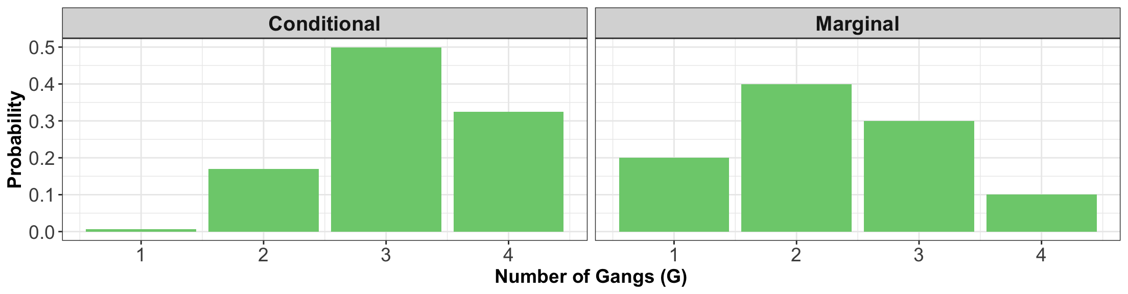
| L = 1 | 0.0068 | 0.1701 | 0.4988 | 0.3242 |
Comparing versus the marginal distribution of the number of \(\text{Gangs}\) \(G\):
| G = 1 | G = 2 | G = 3 | G = 4 | |
|---|---|---|---|---|
| L = 1 | 0.0068 | 0.1701 | 0.4988 | 0.3242 |
| G = 1 | G = 2 | G = 3 | G = 4 |
|---|---|---|---|
| 0.2 | 0.4 | 0.3 | 0.1 |
2.2. Formula Approach
- By applying the formula for conditional probabilities, we get \[P(G = g \mid L = 1) = \frac{P(G = g \cap L = 1)}{P(L = 1)} \quad \text{for } g = 1, 2, 3, 4.\]
| G = 1 | G = 2 | G = 3 | G = 4 | |
|---|---|---|---|---|
| L = 1 | 0.00170 | 0.04253 | 0.12471 | 0.08106 |
| L = 2 | 0.02664 | 0.16981 | 0.13598 | 0.01757 |
| L = 3 | 0.05109 | 0.11563 | 0.03203 | 0.00125 |
| L = 4 | 0.04653 | 0.04744 | 0.00593 | 0.00010 |
| L = 5 | 0.07404 | 0.02459 | 0.00135 | 0.00002 |
Obtaining \(P(L = 1)\)
\[\begin{align*} P(L = 1) &= P(G = 1 \cap L = 1) + P(G = 2 \cap L = 1) + \\ & \qquad P(G = 3 \cap L = 1) + P(G = 4 \cap L = 1) \\ &= 0.0017 + 0.0425 + 0.1247 + 0.0811 \\ &= 0.25. \end{align*}\]
Sanity Check
- The previous four conditional probabilities are part of a proper conditional PMF: \[\begin{align*} \sum_{g = 1}^4 P(G = g \mid L = 1) &= 0.0068 + 0.1701 + \\ & \qquad 0.4988 + 0.3242 \\ &= 1. \end{align*}\]
- Both approaches, table and formula, are equivalent!
Proceeding with the Cargo Ships!
- Suppose we have the following conditional means of gang request \(G\) given the length of stay \(D\) of a ship as a model function:
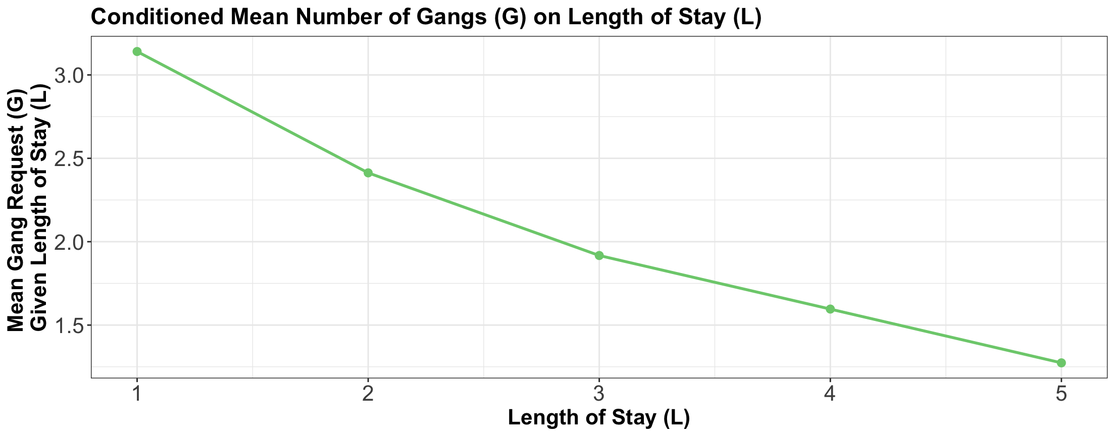
How can we compute \(\mathbb{E}_G(G)\)?
- Multiplying the last two columns together, and summing, gives us the marginal expectation:
\[\begin{align*} \mathbb{E}_G(G) &= \sum_l \mathbb{E}_G(G \mid L = l) \cdot P(L = l) \\ &= 2.3. \end{align*}\]
Let us check an example!

- Let \(L\) be a student’s lab grade in DSCI 551,
- \(Q\) be a student’s quiz grade in DSCI 551, and
- \(S\) represents whether the student majored in Statistics in their undergraduate studies.
Finally…
- Note that we have to repeat the previous checking for the other level combinations of \(L\) and \(Q\) given \(S = \text{yes}\) and \(S = \text{no}\).
- That done, we can conclude the lab grade and quiz grade are not independent, but they are conditionally independent given information about whether the student was a Statistics major.
![]()