Continuous Distributions

Lecture 6

Please, sign in on iClicker

Time to check different continuous families!

Today’s Learning Goals

By the end of this lecture, we will be able to…

• Identify and apply common continuous distribution families.
• Identify what makes a function a bivariate probability density function.
• Compute conditional distributions for continuous random variables.
• Compute conditional distributions for continuous random variables.

Outline

1. Common Continuous Distribution Families
2. Continuous Multivariate Distributions
3. Conditional Distributions (Revisited)

1. Common Continuous Distribution Families

• Just like for discrete distributions, there are also parametric families of continuous distributions.
• Recall the chart of univariate distributions.

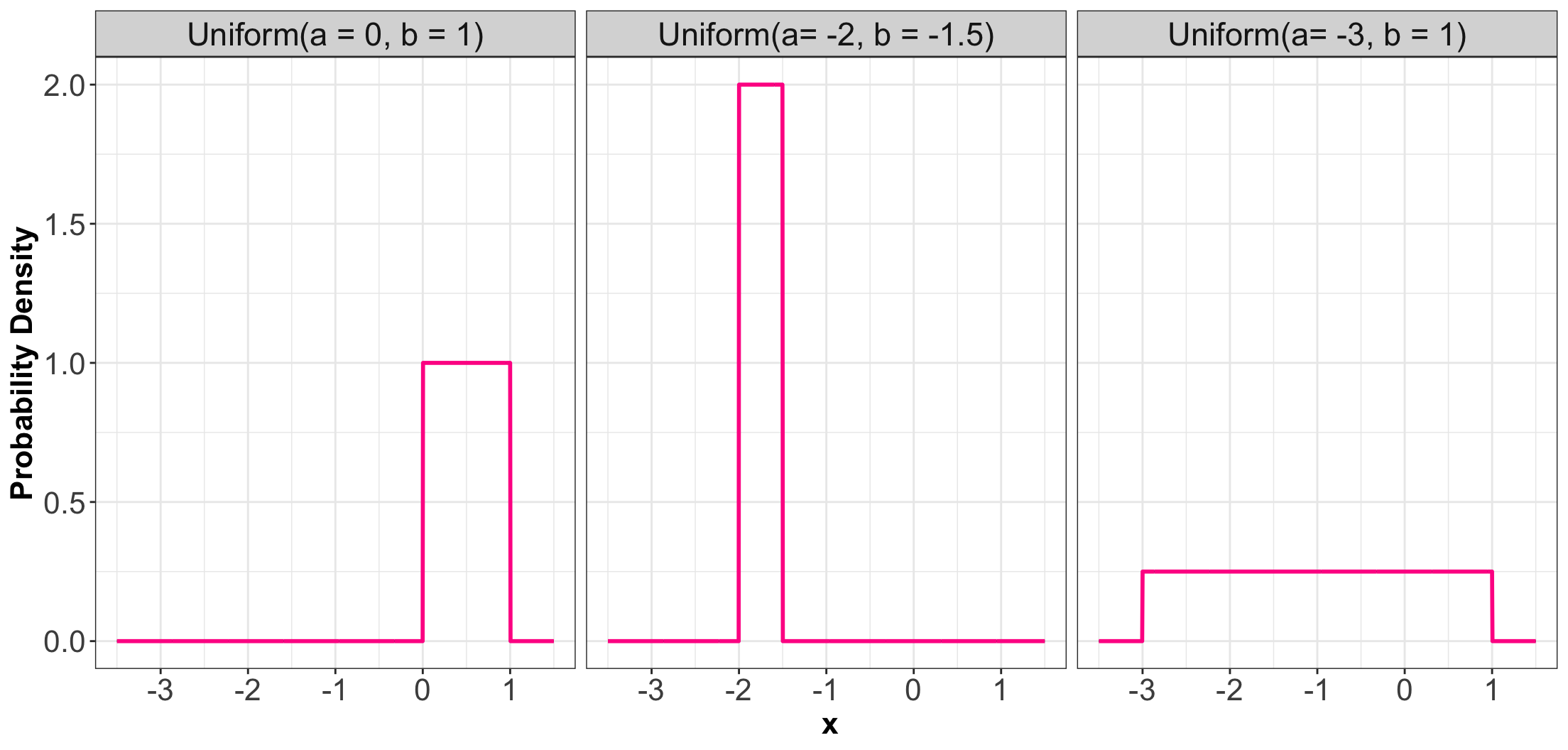
1.1. Uniform

• A Uniform distribution has equal density in between two points \(a\) and \(b\) (for \(a < b\)).
• There are two parameters: one for each end-point.
• Commonly, a reference to a Uniform distribution usually implies continuous uniform.

PDF, Mean, and Variance

• It is denoted as \[X \sim \operatorname{Uniform}(a, b).\]
• The PDF is given by \[f_X(x\mid a, b) = \frac{1}{b - a} \qquad \text{for} \quad a \leq x \leq b.\]
• The mean is \(\mathbb{E}(X) = \frac{a + b}{2}\).
• The variance is \(\text{Var}(X) = \frac{(b - a)^2}{12}\).

Some members of the Uniform family…

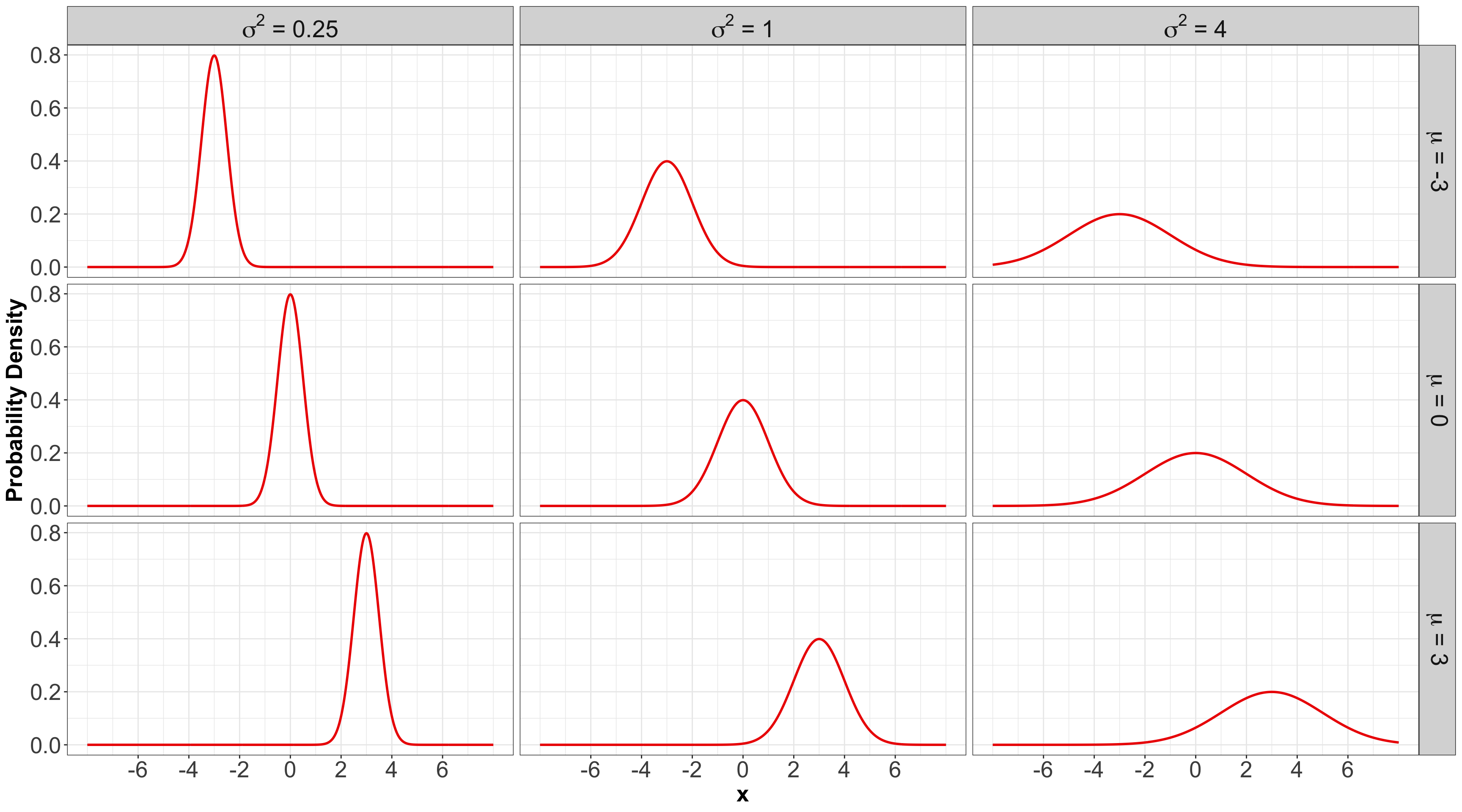
1.2. Gaussian or Normal

• Probably the most famous family of distributions.
• It has a density that follows a “bell-shaped” curve.
• It is parameterized by its mean \[-\infty < \mu < \infty\] and variance \[\sigma^2 > 0.\]

PDF, Mean, and Variance

• It is denoted as \[X \sim \mathcal N\left(\mu, \sigma^2\right).\]
• The PDF is \[f_X(x \mid \mu, \sigma^2) = \frac{1}{\sqrt{2\pi \sigma^2}} \exp \left[-\frac{(x - \mu)^2}{2\sigma^2} \right] \quad \text{for } -\infty < x < \infty.\]
• The mean is \(\mathbb{E}(X) = \mu\).
• The variance is \(\text{Var}(X) = \sigma^2\).

Some members of the Gaussian or Normal family…

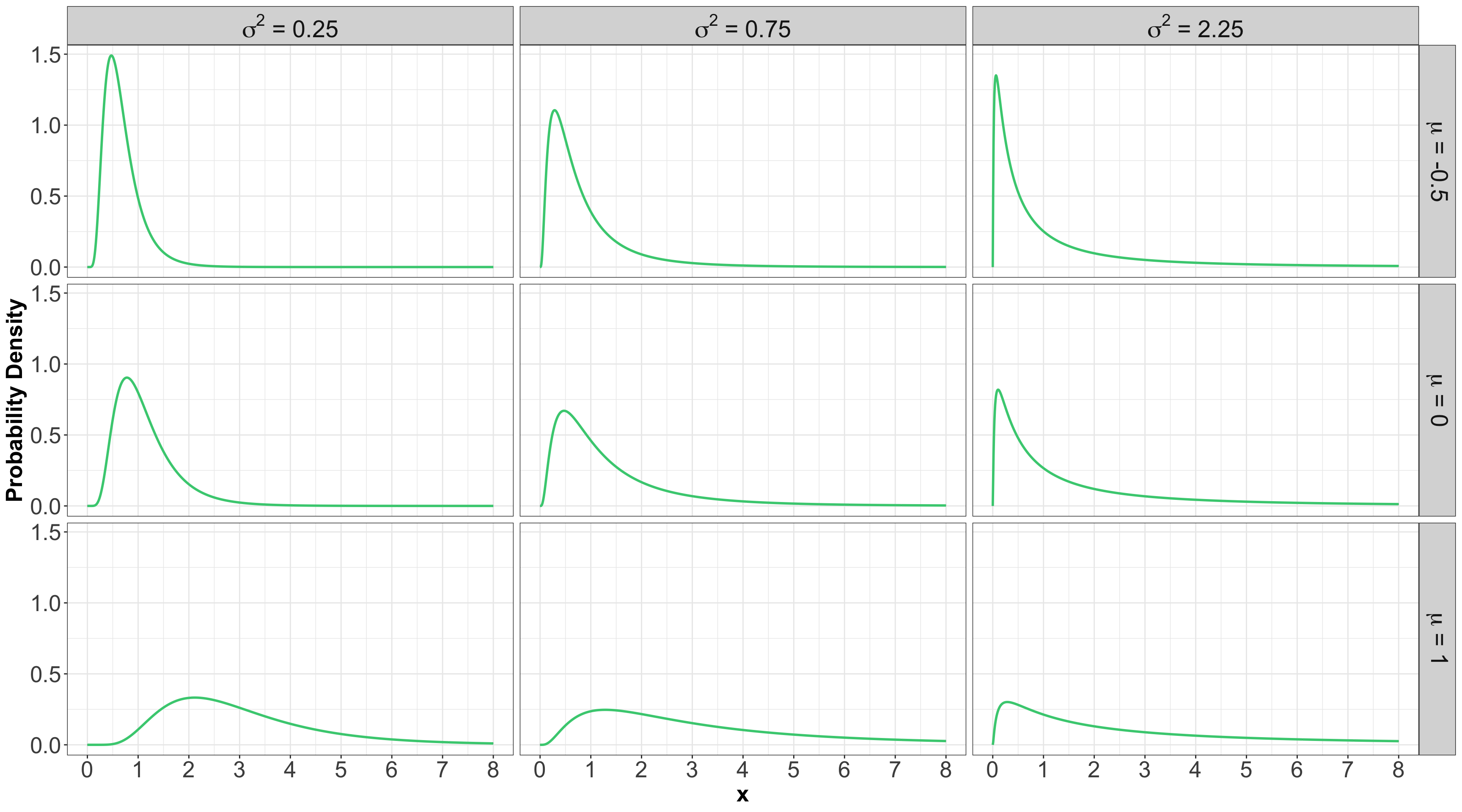
1.3. Log-Normal

• A random variable \(X\) is a Log-Normal distribution if the transformation \(\log(X)\) is Normal.
• This family is often parameterized by the mean \[-\infty < \mu < \infty\] and variance \[\sigma^2 > 0\] of \(\log X\).

PDF, Mean, and Variance

• It is denoted as \[X \sim \operatorname{Log-Normal}\left(\mu, \sigma^2\right).\]
• The PDF is \[f_X(x \mid \mu, \sigma^2) = \frac{1}{x\sqrt{2\pi \sigma^2}} \exp \left\{ -\frac{[\log(x) - \mu]^2}{2\sigma^2} \right\} \quad \text{for } x \geq 0.\]
• The mean is \(\mathbb{E}(X) = \exp{\left[ \mu + \left( \sigma^2 / 2 \right) \right]}\).
• The variance is \(\text{Var}(X) = \exp{\left[ 2 \left( \mu + \sigma^2 \right) \right]} - \exp{\left( 2\mu + \sigma^2 \right)}\).

Some members of the Log-Normal family…

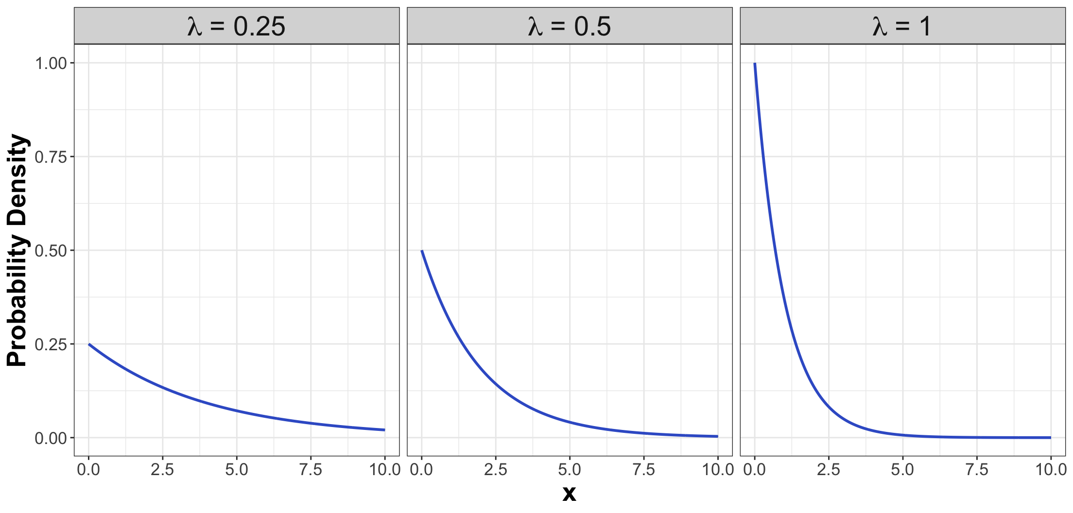
1.4. Exponential

• The Exponential family is for positive random variables.
• It is often interpreted as wait time for some event to happen.
• The family is characterized by a single parameter, usually either the mean wait time \(\beta > 0\), or its reciprocal, the average rate \(\lambda > 0\) at which events happen.

Definition

• The Exponential family is denoted as \[X \sim \operatorname{Exponential}(\beta),\] or \[X \sim \operatorname{Exponential}(\lambda).\]

PDFs

• The PDF can be parameterized as \[f_X(x \mid \beta) = \frac{1}{\beta} \exp(-x / \beta) \qquad \text{for} \quad x \geq 0\] or \[f_X(x \mid \lambda) = \lambda \exp(-\lambda x) \qquad \text{for} \quad x \geq 0.\]

Mean

• Using a \(\beta\) parameterization, the mean is: \[\mathbb{E}(X) = \beta.\]
• On the other hand, using a \(\lambda\) parameterization, the mean is: \[\mathbb{E}(X) = 1 / \lambda.\]

Variance

• Using a \(\beta\) parameterization, the variance is: \[\text{Var}(X) = \beta^2.\]
• On the other hand, using a \(\lambda\) parameterization, the variance is: \[\text{Var}(X) = 1 / \lambda^2.\]

Some members of the Exponential family…

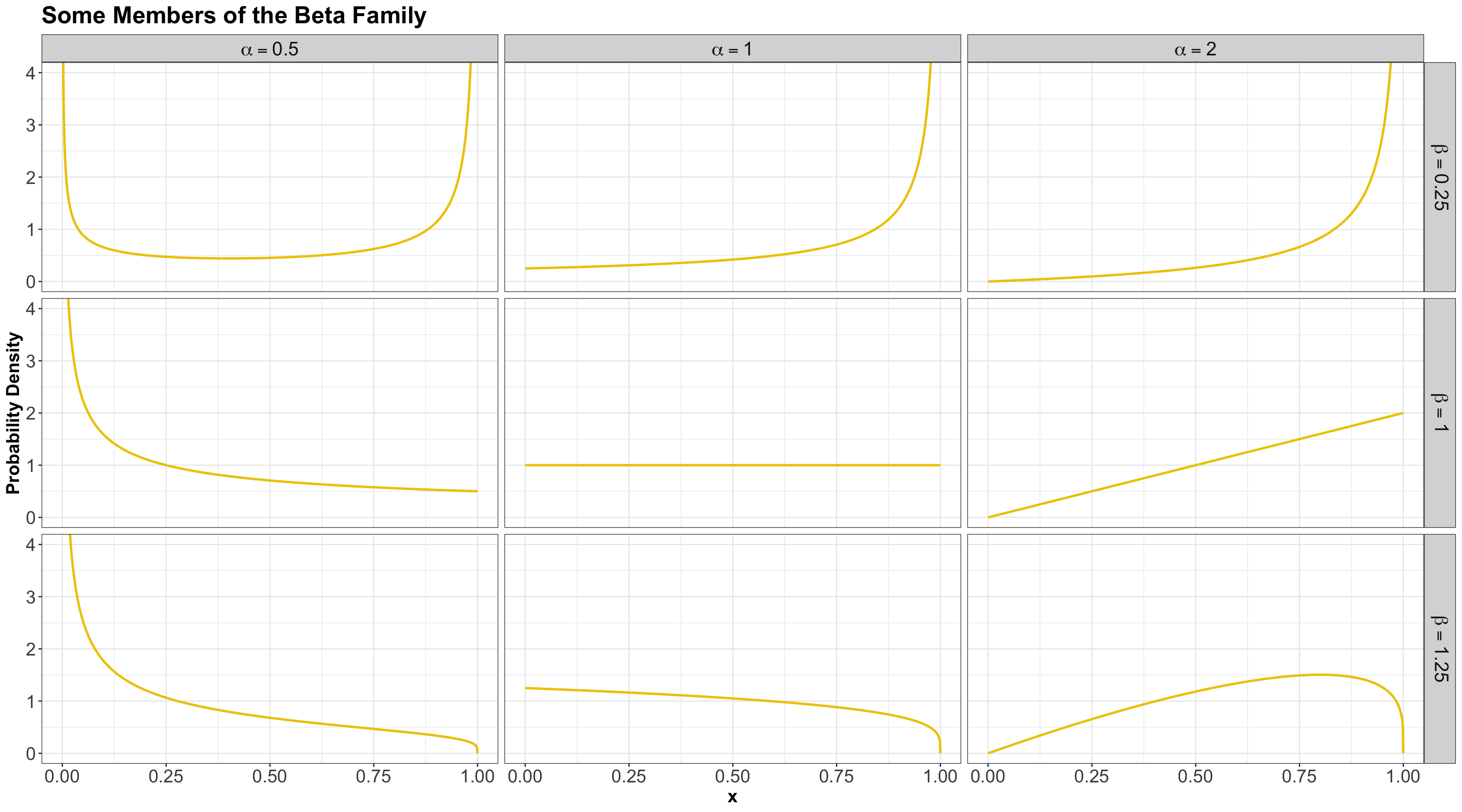
1.5. Beta

• The Beta family of distributions is defined for random variables taking values between \(0\) and \(1\).
• Hence, it is useful for modelling the distribution of proportions.
• It is characterized by two positive shape parameters, \(\alpha > 0\) and \(\beta > 0\).

PDF

• It is denoted as \[X \sim \operatorname{Beta}(\alpha, \beta).\]
• The PDF is given by \[f_X(x \mid \alpha, \beta) = \frac{\Gamma(\alpha + \beta)}{\Gamma(\alpha) \Gamma(\beta)} x^{\alpha - 1} (1 - x)^{\beta - 1} \quad \text{for} \quad 0 \leq x \leq 1,\] where \(\Gamma(\cdot)\) is the Gamma function.

Mean and Variance

• The mean is \[\mathbb{E}(X) = \frac{\alpha}{\alpha + \beta}.\]
• The variance is \[\text{Var}(X) = \frac{\alpha \beta}{(\alpha + \beta)^2 (\alpha + \beta + 1)}.\]

Some members of the Beta family…

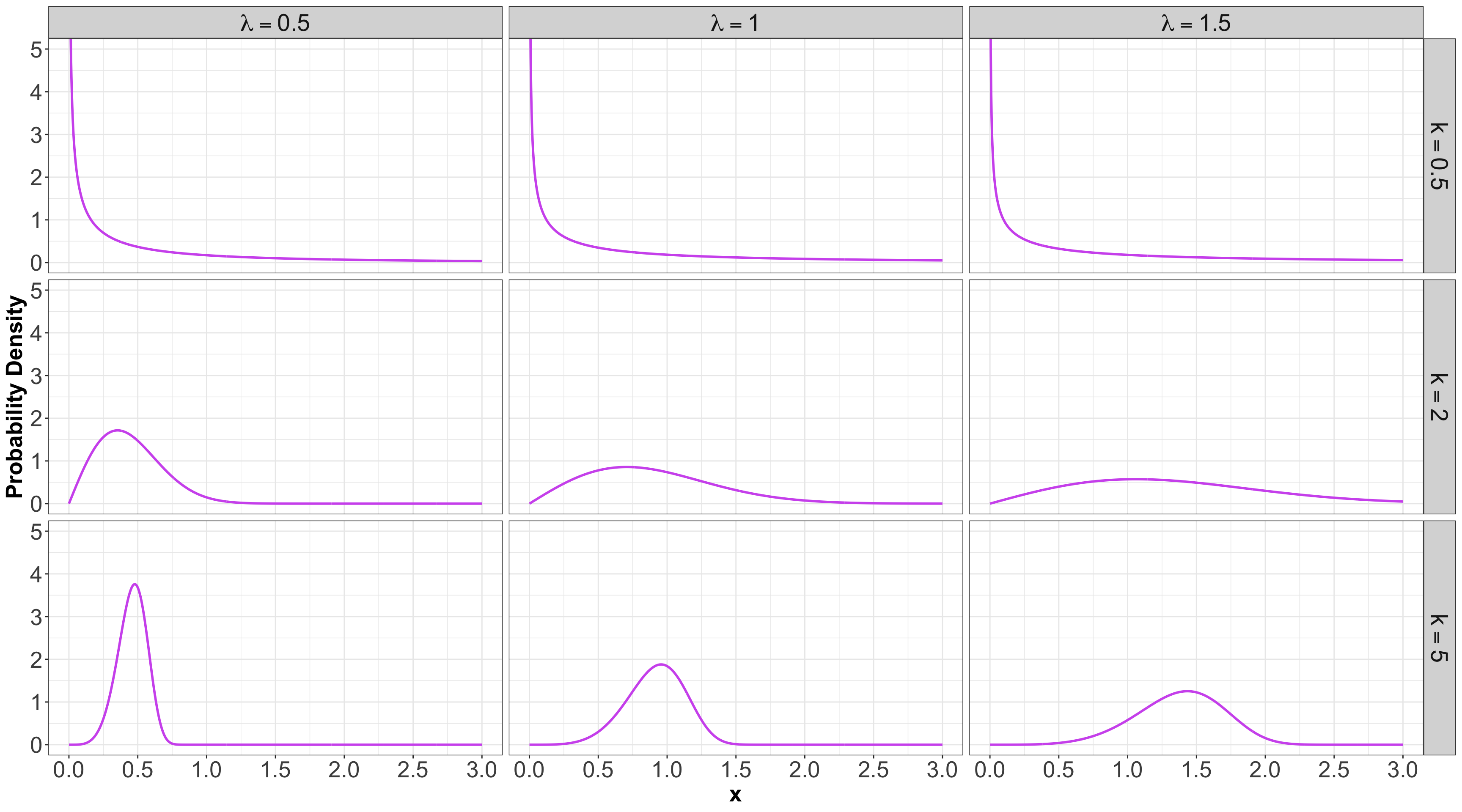
1.6. Weibull

• A generalization of the Exponential family, which allows for an event to be more likely the longer you wait.
• Because of this flexibility and interpretation, this family is used heavily in survival analysis when modelling time until an event.
• This family is characterized by two parameters, a scale parameter \(\lambda > 0\) and a shape parameter \(k > 0\).

PDF

• It is denoted as \[X \sim \operatorname{Weibull}(\lambda, k).\]
• The PDF is \[f_X(x \mid \lambda, k) = \frac{k}{\lambda} \left( \frac{x}{\lambda} \right)^{k - 1} \exp^{-(x / \lambda)^k} \qquad \text{for} \quad x \geq 0.\]

Mean and Variance

• The mean is \[\mathbb{E}(X) = \lambda^{1/k} \Gamma \left( 1 + \frac{1}{k} \right).\]
• The variance is \[\text{Var}(X) = \lambda^{2 / k} \left[ \Gamma \left( 1 + \frac{2}{k} \right) - \Gamma^2 \left( 1 + \frac{1}{k} \right) \right].\]

Some members of the Weibull family…

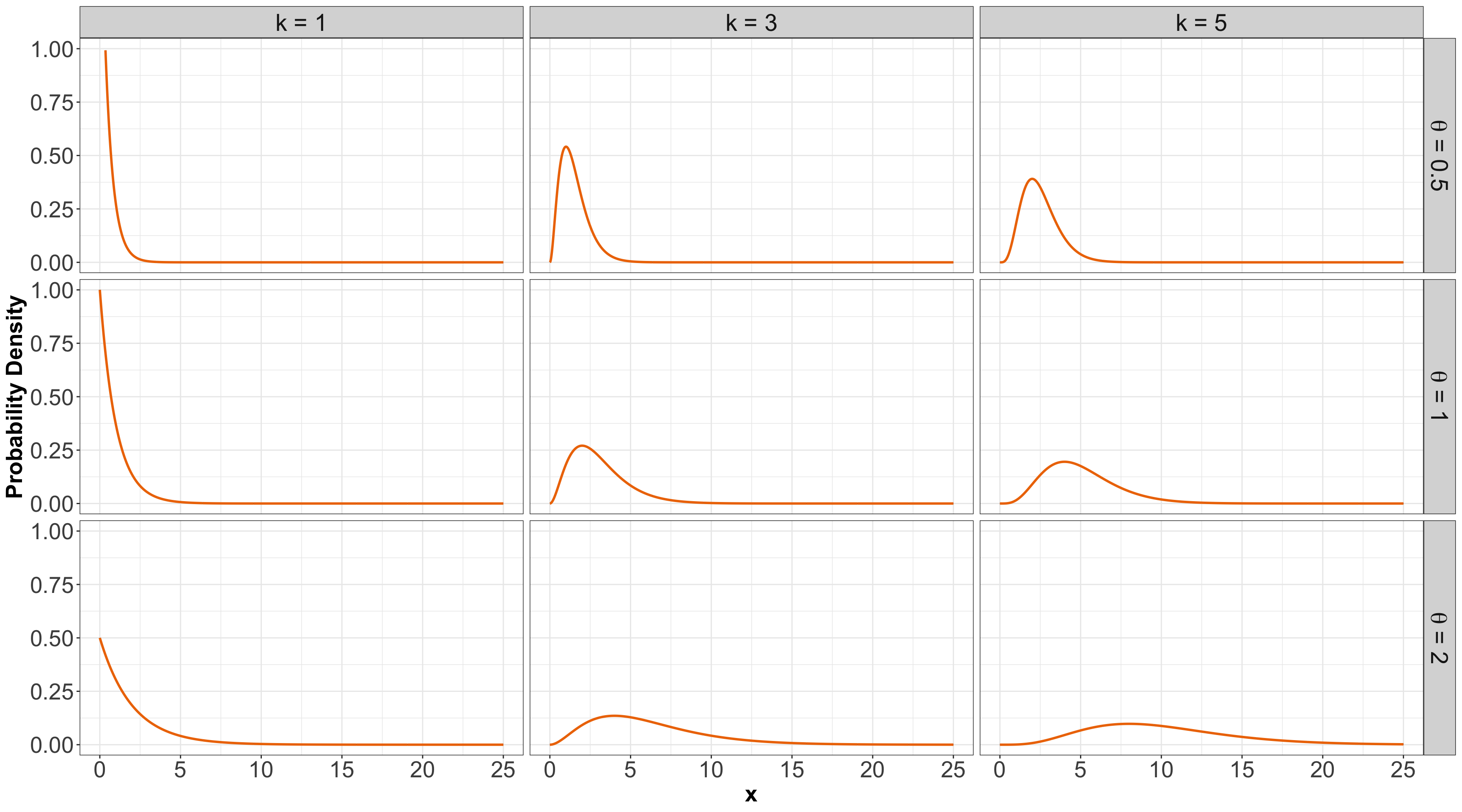
1.7. Gamma

• Another useful two-parameter family with support on non-negative numbers.
• One common parameterization is with a shape parameter \(k > 0\) and a scale parameter \(\theta > 0\).

PDF, Mean, and Variance

• It is denoted as \[X \sim \operatorname{Gamma}(k, \theta).\]
• The PDF is given by \[f_X(x \mid k, \theta) = \frac{1}{\Gamma(k) \theta^k} x^{k - 1} \exp(-x / \theta) \qquad \text{for} \quad x \geq 0,\]
• The mean is \(\mathbb{E}(X) = k \theta\).
• The variance is \(\text{Var}(X) = k \theta^2\).

Some members of the Gamma family…

Summarizing!

1.8 Relevant R Functions

• R has functions for many distribution families.
• The functions are of the form <x><dist>, where <dist> is an abbreviation of a distribution family, and <x> is one of d, p, q, or r.

Possible Prefixes for <x>

• d: density function – we call this \(f_X(x)\).
• p: cumulative distribution function (CDF), we call this \(F_X(x)\).
• q: quantile function (inverse CDF).
• r: random number generator.

Abbreviations for <dist>

• unif: Uniform (continuous).
• norm: Normal (continuous).
• lnorm: Log-Normal (continuous).
• geom: Geometric (discrete).
• pois: Poisson (discrete).
• binom: Binomial (discrete).
• etc.

Examples for <dist>

• For the Uniform family, we have the following R functions:
  • dunif(), punif(), qunif(), and runif().
    
• For the Gaussian or Normal family, we have the following R functions:
  • dnorm(), pnorm(), qnorm(), and rnorm().

iClicker Question

What R function do we need to obtain the density corresponding for \(X \sim \mathcal N(\mu = 2, \sigma^2 = 4)\) at point \(x = 3\)? Select the correct option:

A. pnorm(q = 3, mean = 2, sd = 2)

B. dnorm(x = 3, mean = 2, sd = 4)

C. pnorm(q = 3, mean = 2, sd = 4)

D. dnorm(x = 3, mean = 2, sd = 2)

iClicker Question

What R function do we need for the CDF for \(X \sim \operatorname{Uniform}(a = 0, b = 2)\) at \(x = 0.25, 0.5, 0.75\)?

A. qunif(p = c(0.25, 0.5, 0.75), min = 0, max = 2, lower.tail = TRUE)

B. punif(q = c(0.25, 0.5, 0.75), min = 0, max = 2, lower.tail = TRUE)

C. dunif(x = c(0.25, 0.5, 0.75), min = 0, max = 2)

D. punif(q = c(0.25, 0.5, 0.75), min = 0, max = 2, lower.tail = FALSE)

iClicker Question

What R function do we need to obtain the median of \(X \sim \operatorname{Uniform}(a = 0, b = 2)\)?

A. qunif(p = 0.5, min = 0, max = 2, lower.tail = TRUE)

B. punif(q = 0.5, min = 0, max = 2, lower.tail = TRUE)

C. dunif(x = 0.5, min = 0, max = 2)

D. punif(q = 0.5, min = 0, max = 2, lower.tail = FALSE)

iClicker Question

What R function do we need to generate a random sample of size \(10\) from the distribution \(\mathcal N(\mu = 0, \sigma^2 = 25)\)?

A. runif(n = 10, min = 0, max = 25)

B. rnorm(n = 10, mean = 0, sd = 25)

C. rnorm(n = 10, mean = 0, sd = 5)

D. runif(n = 10, min = 0, max = 5)

2. Continuous Multivariate Distributions

• In the discrete case we already saw joint distributions, conditional distributions, marginal distributions, etc.
• All these concepts are carried over to the continuous world.
• Let us start with two continuous variables (i.e., a bivariate case).

2.1. Continuous Multivariate Distributions

• Recall the joint probability mass function (PMF) between \(\text{Gang}\) demand and length-of-stay in days (\(\text{LOS}\)):

	Gangs = 1	Gangs = 2	Gangs = 3	Gangs = 4
LOS = 1	0.00170	0.04253	0.12471	0.08106
LOS = 2	0.02664	0.16981	0.13598	0.01757
LOS = 3	0.05109	0.11563	0.03203	0.00125
LOS = 4	0.04653	0.04744	0.00593	0.00010
LOS = 5	0.07404	0.02459	0.00135	0.00002

How can we set up a joint PDF?

• Suppose you have two continuous random variables that have a joint PDF.
• For this continuous case, instead of rows and columns, we have an \(x\) and \(y\)-axis for our two random variables, defining a region of possible values.

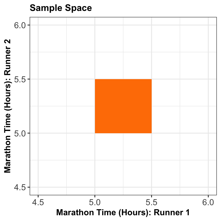
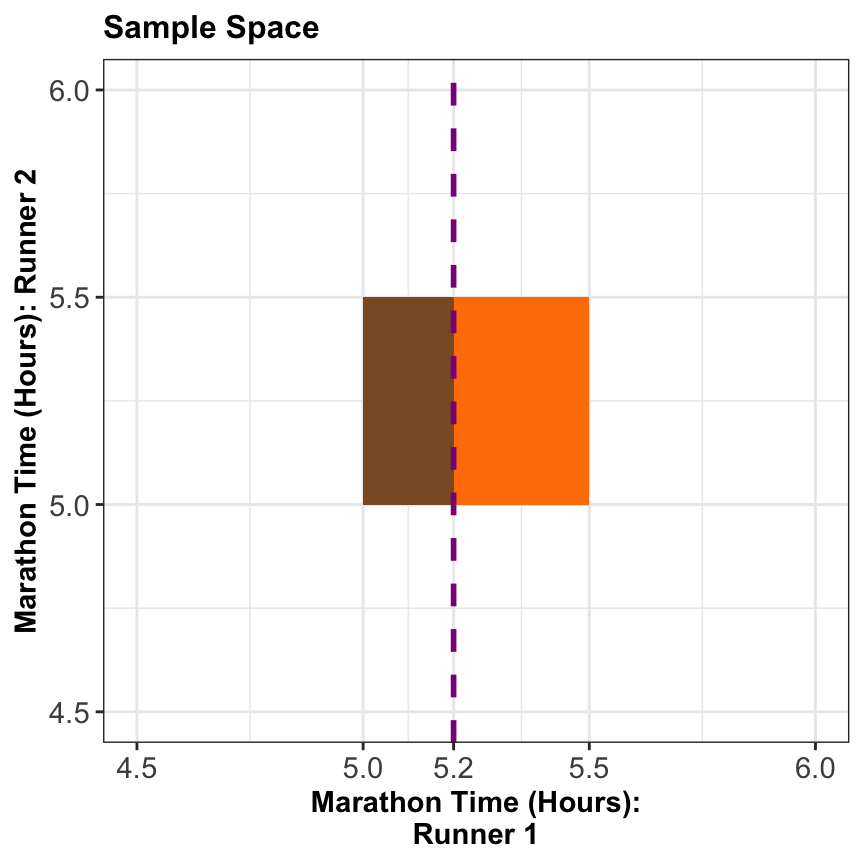
The two-runner example!

• Suppose two marathon runners can only finish a marathon between 5.0 and 5.5 hours each, and their end times are totally random!

A bivariate density function in 3D!

• The density function is a surface overtop of this square.
• The orange distribution surface corresponds to the projection of the joint distribution on the \(z\)-axis.

2.2. Calculating Probabilities

• Let \(X\) and \(Y\) be two random variables. Their joint PDF evaluated at the points \(x\) and \(y\) is usually denoted \[f_{X,Y}(x,y).\]
• Therefore, we have a density surface.
• We can calculate probabilities as the volume under the density surface.

What do we mean when we say a “volume”?

• The total volume under the density function must equal 1.
• Formally, this may be written as \[\int_{-\infty}^{\infty} \int_{-\infty}^{\infty} f_{X, Y} (x,y)\,\mathrm{d}x\,\mathrm{d}y = 1.\]

In-Class Question

• In the two-runner example, if the density is equal/flat across the entire sample space, what is the height of this surface?
• That is, what does the density evaluate to?
• What does it evaluate to outside of the sample space?

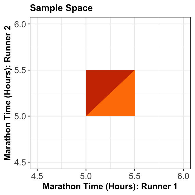
In-Class Question

• Let \(X\) and \(Y\) be the marathon times of Runner 1 and Runner 2 in hours, respectively.
• What is the probability that Runner 1 will finish the marathon before Runner 2, i.e., \(P(X < Y)\)?

In-Class Question

• What is the probability that Runner 1 finishes in \(5.2\) hours or less, i.e., \(P(X \leq 5.2)\)?

3. Conditional Distributions (Revisited)

• Recall the basic formula for conditional probabilities for events \(A\) and \(B\):

\[P(A \mid B) = \frac{P(A \cap B)}{P(B)}.\]

• Nonetheless, this is only true if \(P(B) \neq 0\), and it is not useful if \(P(A) = 0\) – two situations we are faced with in the continuous world!

3.1. When \(P(A) = 0\)

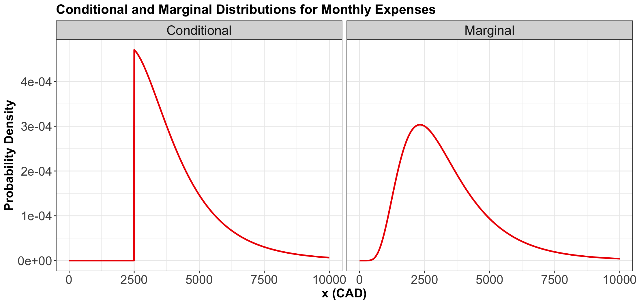
• Suppose the month is half-way over, and you find that you only have \(\$2500\) worth of expenses so far!
• What is the distribution of this month’s total expenditures now, given this information?

Applying the previous Law of Conditional Probability…

• Let \[X = \text{Monthly Expenses in CAD}.\]
• Assume \[X \sim \operatorname{Log-Normal}(\mu = 8, \sigma^2 = 0.5).\]
• Using the conditional probability formula would give: \[P(X = x \mid X \geq 2500) = \frac{P(X = x)}{P(X \geq 2500)} \qquad \qquad \text{(NO!)}\]

Instead…

• In general, we replace probabilities with densities.
• In this case, what we actually have is: \[f_{X \mid X \geq 2500}(x) = \frac{f_X(x)}{P(X \geq 2500)} \qquad \text{for} \quad x \geq 2500,\] and \[f_{X \mid X \geq 2500}(x) = 0 \qquad \text{for} \quad x < 2500.\]

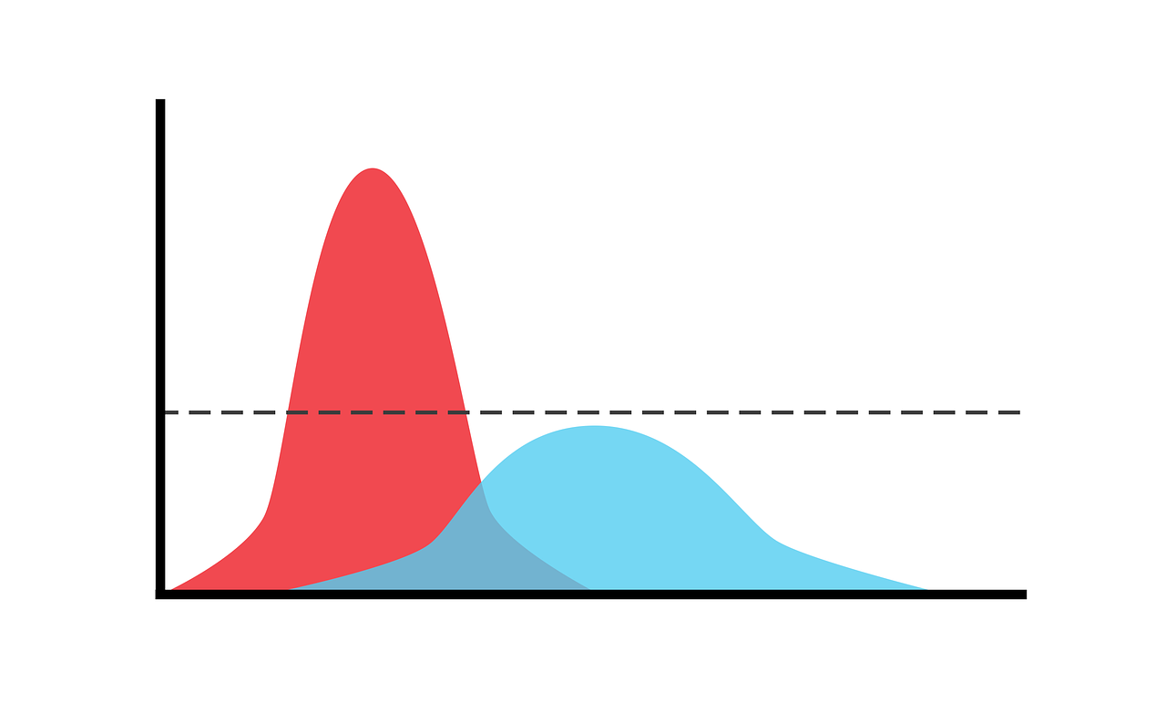
Comparing Densities

3.2. When \(P(B) = 0\)

• To describe this situation, let us use the marathon runners’ example again:

If Runner 1 ended up finishing in \(5.2\) hours, what is the distribution of Runner 2’s time?

• Let \(X\) be the time for Runner 1, and \(Y\) for Runner 2, what we are asking for is \[f_{Y|X = 5.2}(y).\]

However…

• We already pointed out that \(P(X = 5.2) = 0.\)

• We end up with: \[f_{Y|X = 5.2}(y) = \frac{f_{Y,X}(y, 5.2)}{f_X(5.2)}.\]
• This formula is true in general: \[f_{Y|X}(y) = \frac{f_{Y,X}(y, x)}{f_X(x)}.\]