DSCI_562_regr-2
GLM’s in R
This document introduces the glm() function in R for fitting a Generlized Linear Model (GLM). We’ll work with the titanic_train dataset in the titanic package.
library(tidyverse)
## ── Attaching packages ────────────────────────────────────────────────────────────── tidyverse 1.2.1 ──

## ✔ ggplot2 3.1.0     ✔ purrr   0.2.5
## ✔ tibble  1.4.2     ✔ dplyr   0.7.6
## ✔ tidyr   0.8.1     ✔ stringr 1.3.1
## ✔ readr   1.1.1     ✔ forcats 0.3.0

## ── Conflicts ───────────────────────────────────────────────────────────────── tidyverse_conflicts() ──
## ✖ dplyr::filter() masks stats::filter()
## ✖ dplyr::lag()    masks stats::lag()
library(broom)
library(titanic)
dat <- na.omit(titanic_train)
str(dat)
## 'data.frame':    714 obs. of  12 variables:
##  $ PassengerId: int  1 2 3 4 5 7 8 9 10 11 ...
##  $ Survived   : int  0 1 1 1 0 0 0 1 1 1 ...
##  $ Pclass     : int  3 1 3 1 3 1 3 3 2 3 ...
##  $ Name       : chr  "Braund, Mr. Owen Harris" "Cumings, Mrs. John Bradley (Florence Briggs Thayer)" "Heikkinen, Miss. Laina" "Futrelle, Mrs. Jacques Heath (Lily May Peel)" ...
##  $ Sex        : chr  "male" "female" "female" "female" ...
##  $ Age        : num  22 38 26 35 35 54 2 27 14 4 ...
##  $ SibSp      : int  1 1 0 1 0 0 3 0 1 1 ...
##  $ Parch      : int  0 0 0 0 0 0 1 2 0 1 ...
##  $ Ticket     : chr  "A/5 21171" "PC 17599" "STON/O2. 3101282" "113803" ...
##  $ Fare       : num  7.25 71.28 7.92 53.1 8.05 ...
##  $ Cabin      : chr  "" "C85" "" "C123" ...
##  $ Embarked   : chr  "S" "C" "S" "S" ...
##  - attr(*, "na.action")= 'omit' Named int  6 18 20 27 29 30 32 33 37 43 ...
##   ..- attr(*, "names")= chr  "6" "18" "20" "27" ...
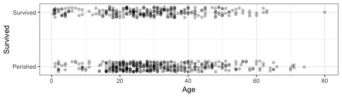
Consider the regression of Survived on Age. Let’s take a look at the data with jitter:
ggplot(dat, aes(Age, Survived)) +
    geom_jitter(height=0.1, alpha=0.25) +
    scale_y_continuous(breaks=0:1, labels=c("Perished", "Survived")) +
    theme_bw()
Recall that the linear regression can be done with the lm function:
res_lm <- lm(Survived ~ Age, data=dat)
summary(res_lm)
##
## Call:
## lm(formula = Survived ~ Age, data = dat)
##
## Residuals:
##     Min      1Q  Median      3Q     Max
## -0.4811 -0.4158 -0.3662  0.5789  0.7252
##
## Coefficients:
##              Estimate Std. Error t value Pr(>|t|)
## (Intercept)  0.483753   0.041788  11.576   <2e-16 ***
## Age         -0.002613   0.001264  -2.067   0.0391 *
## ---
## Signif. codes:  0 '***' 0.001 '**' 0.01 '*' 0.05 '.' 0.1 ' ' 1
##
## Residual standard error: 0.4903 on 712 degrees of freedom
## Multiple R-squared:  0.005963,   Adjusted R-squared:  0.004567
## F-statistic: 4.271 on 1 and 712 DF,  p-value: 0.03912
In this case, the regression line is 0.4837526 + -0.0026125 Age.
A GLM can be fit in a similar way, using the glm function – we just need to indicate what type of regression we’re doing (binomial? poission?) and the link function. We are doing bernoulli (binomial) regression, since the response is binary (0 or 1); lets choose a probit link function.
res_glm <- glm(factor(Survived) ~ Age, data=dat, family=binomial(link="probit"))
The family argument takes a function, indicating the type of regression. See ?family for the various types of regression allowed by glm().
Let’s see a summary of the GLM regression:
summary(res_glm)
##
## Call:
## glm(formula = factor(Survived) ~ Age, family = binomial(link = "probit"),
##     data = dat)
##
## Deviance Residuals:
##     Min       1Q   Median       3Q      Max
## -1.1477  -1.0363  -0.9549   1.3158   1.5929
##
## Coefficients:
##              Estimate Std. Error z value Pr(>|z|)
## (Intercept) -0.037333   0.107944  -0.346   0.7295
## Age         -0.006773   0.003294  -2.056   0.0397 *
## ---
## Signif. codes:  0 '***' 0.001 '**' 0.01 '*' 0.05 '.' 0.1 ' ' 1
##
## (Dispersion parameter for binomial family taken to be 1)
##
##     Null deviance: 964.52  on 713  degrees of freedom
## Residual deviance: 960.25  on 712  degrees of freedom
## AIC: 964.25
##
## Number of Fisher Scoring iterations: 4
We can make predictions too, but this is not as straight-forward as in lm() – here are the “predictions” using the predict() generic function:
pred <- predict(res_glm)
qplot(dat$Age, pred) + labs(x="Age", y="Default Predictions")
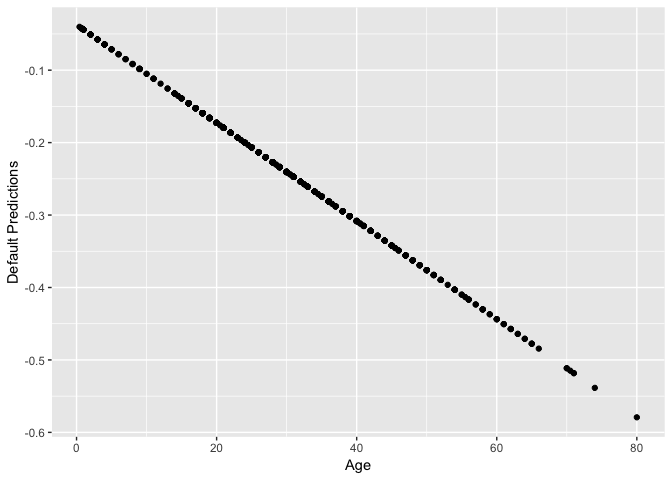
Why the negative predictions? It turns out this is just the linear predictor, -0.0373331 + -0.0067733 Age.
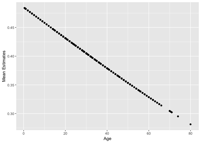
The documentation for the predict() generic function on glm objects can be found by typing ?predict.glm. Notice that the predict() generic function allows you to specify the type of predictions to be made. To make predictions on the mean (probability of Survived=1), indicate type="response", which is the equivalent of applying the inverse link function to the linear predictor.
Here are those predictions again, this time indicating type="response":
pred <- predict(res_glm, type="response")
qplot(dat$Age, pred) + labs(x="Age", y="Mean Estimates")
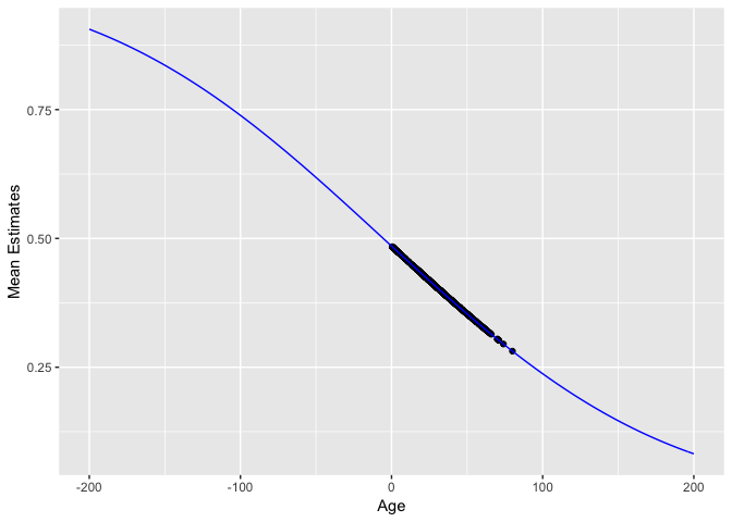
Look closely – these predictions don’t actually fall on a straight line. They follow an inverse probit function (i.e., a Gaussian cdf):
mu <- function(x) pnorm(res_glm$coefficients[1] + res_glm$coefficients[2] * x)
qplot(dat$Age, pred) +
    labs(x="Age", y="Mean Estimates") +
    stat_function(fun=mu, colour="blue") +
    scale_x_continuous(limits=c(-200, 200))
broom::augment()
We can use the broom package on glm objects, too. But, just like we had to specify type="response" when using the predict() function in order to evaluate the model function, so to do we have to specify something in the broom::augment() function. Here, the type.predict argument gets passed to the predict() generic function (actually, the predict.glm() method). This means that indicating type.predict="response" will evaluate the model function:
res_glm %>%
  augment(type.predict = "response") %>%
  head()
## # A tibble: 6 x 10
##   .rownames factor.Survived.   Age .fitted .se.fit .resid    .hat .sigma
##   <chr>     <fct>            <dbl>   <dbl>   <dbl>  <dbl>   <dbl>  <dbl>
## 1 1         0                   22   0.426  0.0209 -1.05  0.00179   1.16
## 2 2         1                   38   0.384  0.0211  1.38  0.00188   1.16
## 3 3         1                   26   0.415  0.0190  1.33  0.00149   1.16
## 4 4         1                   35   0.392  0.0196  1.37  0.00160   1.16
## 5 5         0                   35   0.392  0.0196 -0.997 0.00160   1.16
## 6 7         0                   54   0.343  0.0345 -0.917 0.00528   1.16
## # ... with 2 more variables: .cooksd <dbl>, .std.resid <dbl>