Lecture 1

GLMs: Link Functions and Count Regression

(Please, sign in on iClicker)

Hello and welcome!

Teaching Team

Section 1: Payman Nickchi

Section 2: G. Alexi Rodríguez-Arelis

High-Level Goals of this Course

• Describe the risk and value of making parametric assumptions in regression.
• Fit model functions that represent probabilistic quantities besides the mean.
• Identify situations where Ordinary Least-squares (OLS) regression is sub-optimal, and apply alternative regression methods that better address the situation.

Today’s Learning Goals

By the end of this lecture, you should be able to:

• Explain the Data Science workflow in Regression Analysis.
• Recall the basics of OLS regression.
• Identify cases where OLS regression is not suitable.
• Distinguish what makes a regression model “linear.”
• Explain the concept of generalized linear models (GLMs).
• Explore the concept of the link function.

Today’s Learning Goals (cont’d)

• Outline the modelling framework of count regression.
• Fit and interpret count regression.
• Use count regression for prediction.
• Explain and test overdispersion on count-type data.

Outline

1. A Preamble on our Data Science Workflow
2. Review of Ordinary Least-squares Regression
3. Link Function
4. Poisson Regression
5. Overdispersion
6. Negative Binomial Regression

1. A Preamble on our Data Science Workflow

We have structured this regression course in three big pillars:

1. The use of an ordered Data Science workflow,
2. Choosing the proper workflow flavour according to either an inferential or predictive paradigm.
3. The correct use of an appropriate regression model based on the response of interest.

What is this workflow?

Stages

1. Study design.
2. Data collection and wrangling.
3. Exploratory data analysis.
4. Data modelling.
5. Estimation.
6. Results.
7. Storytelling.

Data Modelling

In Regression Analysis, we can model an unbounded continuous response in terms of their global conditioned mean using OLS for inference or prediction.

2. Review of Ordinary Least-squares Regression

• In DSCI 561, you learned comprehensive material about OLS regression. The term ordinary refers to a linear model with a response of continuous nature : a variable can take on an infinite number of real values in a given range.

• This response might be subject to regressors of a continuous or discrete nature. When the regressors are discrete and factor-type (i.e., with different categories), they could be: nominal or ordinal .

Conceptually…

• A linear regression model can be expressed as:

\[\begin{equation*} \mbox{Response} = \mbox{Systematic Component} + \mbox{Random Component}. \end{equation*}\]

• For the \(i\)th observation in our sample or training data \((i = 1, \dots, n)\), the conceptual model is mathematically represented as:

\[ \underbrace{Y_i}_\text{Response} = \underbrace{\beta_0 + \beta_1 g_1(X_{i, 1}) + \ldots + \beta_k g_k(X_{i,k})}_\text{Systematic Component} + \underbrace{\varepsilon_i}_\text{Random Component} \]

Note the following!

• The response \(Y_i\) is equal to the sum of \(k + 2\) terms.
• The systematic component is the sum of:
  • An unknown intercept \(\beta_0\) and
  • \(k\) regressor functions \(g_j(X_{i,j})\) multiplied by their respective unknown regression coefficient \(\beta_j\) \((j = 1, \dots, k)\).

Moreover…

• \(\varepsilon_i\) is the random noise under the following assumptions: \[\begin{gather*} \mathbb{E}(\varepsilon_i) = 0 \\ \text{Var}(\varepsilon_i) = \sigma^2 \\ \varepsilon_i \sim \mathcal{N}(0, \sigma^2) \\ \varepsilon_i \perp \!\!\! \perp \varepsilon_k \; \; \; \; \text{for} \; i \neq k \; \; \; \; \text{(independence)}. \end{gather*}\]
• Hence, each \(Y_i\) is also assumed to be independent and normally distributed: \[\begin{equation*} Y_i \mid X_{i, j} \sim \mathcal{N} \big( \beta_0 + \beta_1 g_1(X_{i, 1}) + \ldots + \beta_p g_p(X_{i,p}), \sigma^2 \big). \end{equation*}\]

2.1. Can We Apply Linear Regression Here?

Having briefly discussed the components of the OLS model, let us explore three 2-\(d\) examples made with simulated data.

iClicker Question

In what example(s) can we apply linear regression?

A. Examples 1 and 2.

B. Example 1.

C. Examples 1 and 3.

D. Examples 1, 2, and 3.

2.2. What makes a regression model “linear”?

Let us retake the Example 3 from our previous activity.

Data Generation

• Each synthetic data point was generated from a sinusoidal curve plus some normally distributed random noise: \[\begin{align*} Y_i &= \beta_0 + \beta_1 g(X_i) + \varepsilon_i \\ &= \beta_0 + \beta_1 \sin(X_i) + \varepsilon_i. \end{align*}\]

• Hence, this example can be modeled as an OLS model if we transform each observed \(x_i\) in the training set as \(\sin(x_i)\).

In general…

• OLS implicates the identity function \(g_j(X_{i, j}) = X_{i, j}\), leading to:

\[\begin{align*} Y_i &= \beta_0 + \beta_1 g_1(X_{i, 1}) + \ldots + \beta_k g_k(X_{i,}) + \varepsilon_i \\ &= \beta_0 + \beta_1 X_{i,1} + \ldots + \beta_k X_{i,} + \varepsilon_i. \end{align*}\]

3. Link Function

• OLS regression models the following:

\[ \begin{align*} \mu_i &= \mathbb{E}(Y_i \mid X_{i,1}, \ldots, X_{i,k}) \\ &= \beta_0 + \beta_1 X_{i,1} + \ldots + \beta_k X_{i,k} \\ & \qquad \qquad \qquad \qquad \qquad \text{since} \; \; \mathbb{E}(\varepsilon_i) = 0. \end{align*} \]

Nonetheless…

• Modelling the mean \(\mu_i\) of a discrete-type response is not straightforward.
• Hence, we rely on a monotonic and differentiable function \(h(\mu_i)\) called the link function:

\[ \begin{align*} h(\mu_i) &= \eta_i \\ &= \beta_0 + \beta_1 X_{i,1} + \beta_2 X_{i,2} + \ldots + \beta_k X_{i,k} \\ & \qquad \qquad \qquad \qquad \qquad \text{for} \; i = 1, \ldots, n. \end{align*} \]

Why monotonic and differentiable?

• The link function needs to be monotonic so we can allow putting the systematic component \(\eta_i\) in terms of the corresponding mean \(\mu_i\), i.e.:

\[\mu_i = h^{-1}(\eta_i).\]

• It needs to be differentiable since we rely on maximum likelihood estimation to obtain \(\hat{\beta}_0, \hat{\beta}_1, \dots, \hat{\beta}_k\).

Here comes the GLM!

• A GLM has the components of the conceptual regression model in a training set of \(n\) elements as:

1. Random component: Each response \(Y_1,\ldots,Y_n\) is a random variable with mean \(\mu_i\).
2. Systematic component: \[\eta_i = \beta_0 + \beta_1 X_{i,1} + \beta_2 X_{i,2} + \ldots + \beta_k X_{i,k} \; \; \; \; \text{for} \; i = 1, \ldots, n.\]
3. Link function: \[ h(\mu_i) = \eta_i. \]

4. Poisson Regression

4.1. The Crabs Dataset

• The data frame crabs (Brockmann, 1996) is a dataset detailing the counts of satellite male crabs residing around a female crab nest.

Let us take a look at the dataset!

• Beforehand, we do some quick data wrangling.
• Then, we display the first eight rows.

data(crabs)
crabs <- crabs |>
  rename(n_males = satell) |>
  dplyr::select(-y)
head(crabs, n = 8) 

   color  spine width n_males weight
1 medium    bad  28.3       8   3050
2   dark    bad  22.5       0   1550
3  light   good  26.0       9   2300
4   dark    bad  24.8       0   2100
5   dark    bad  26.0       4   2600
6 medium    bad  23.8       0   2100
7  light   good  26.5       0   2350
8   dark middle  24.7       0   1900

Main Statistical Inquiries

Let us suppose we want to assess the following:

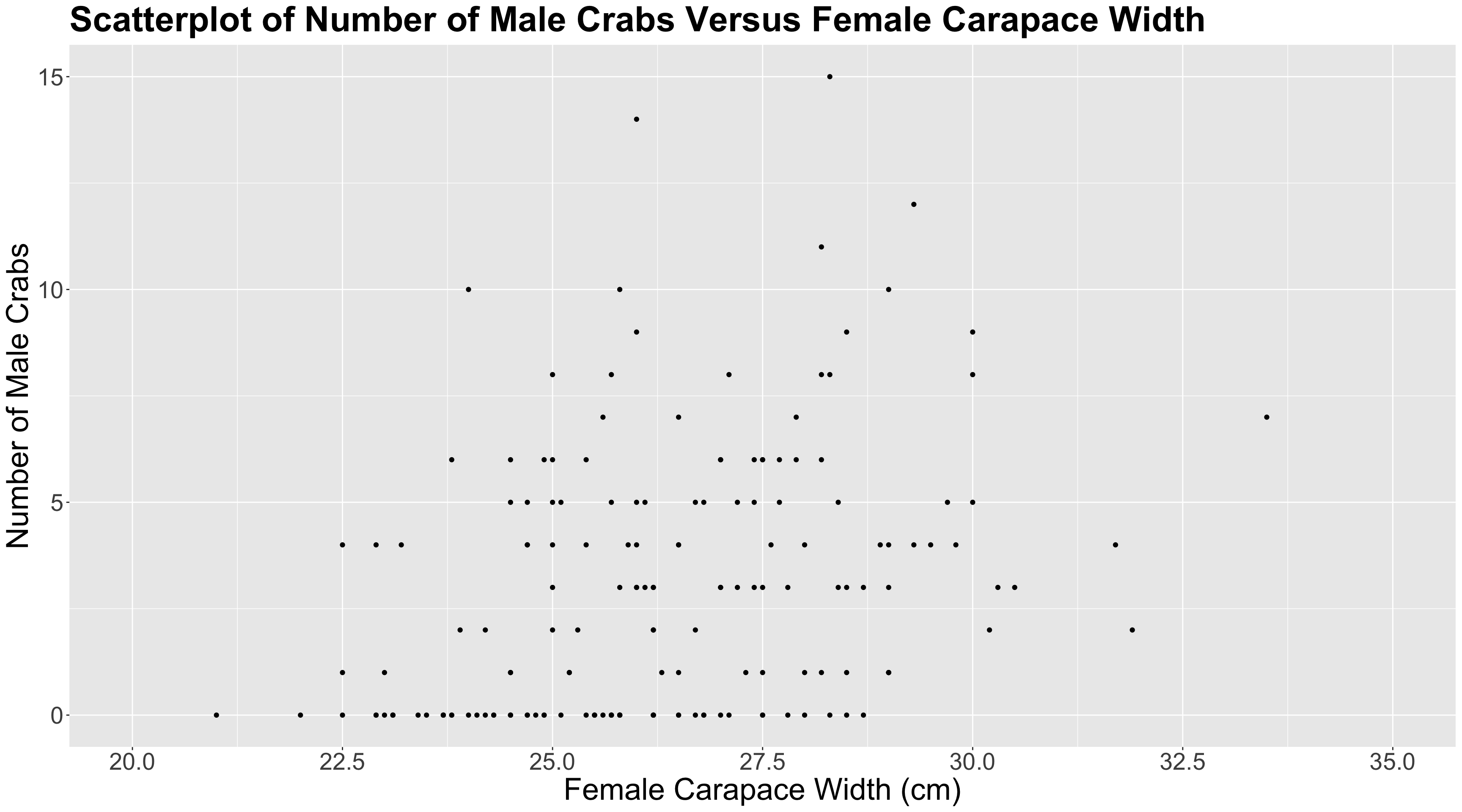
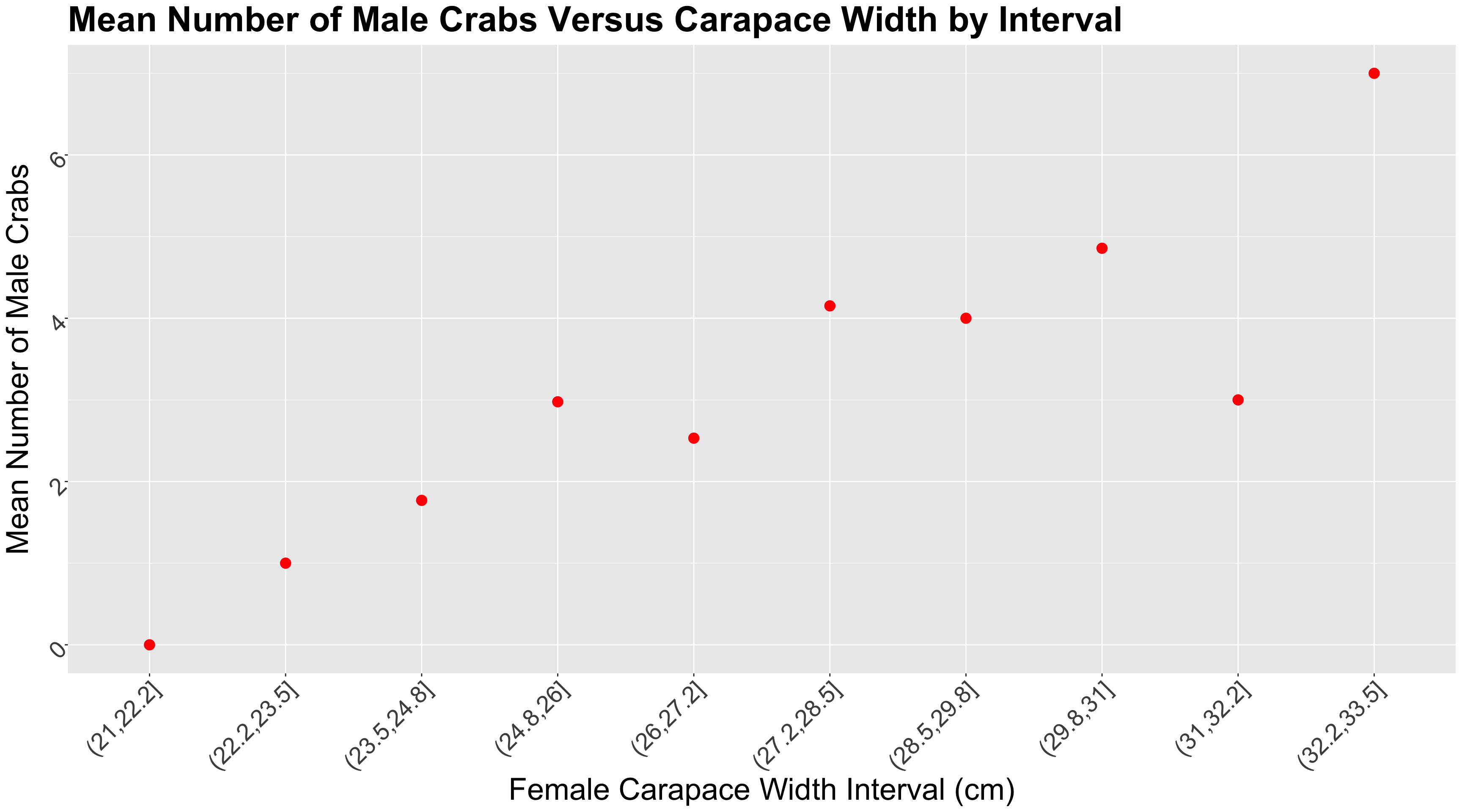
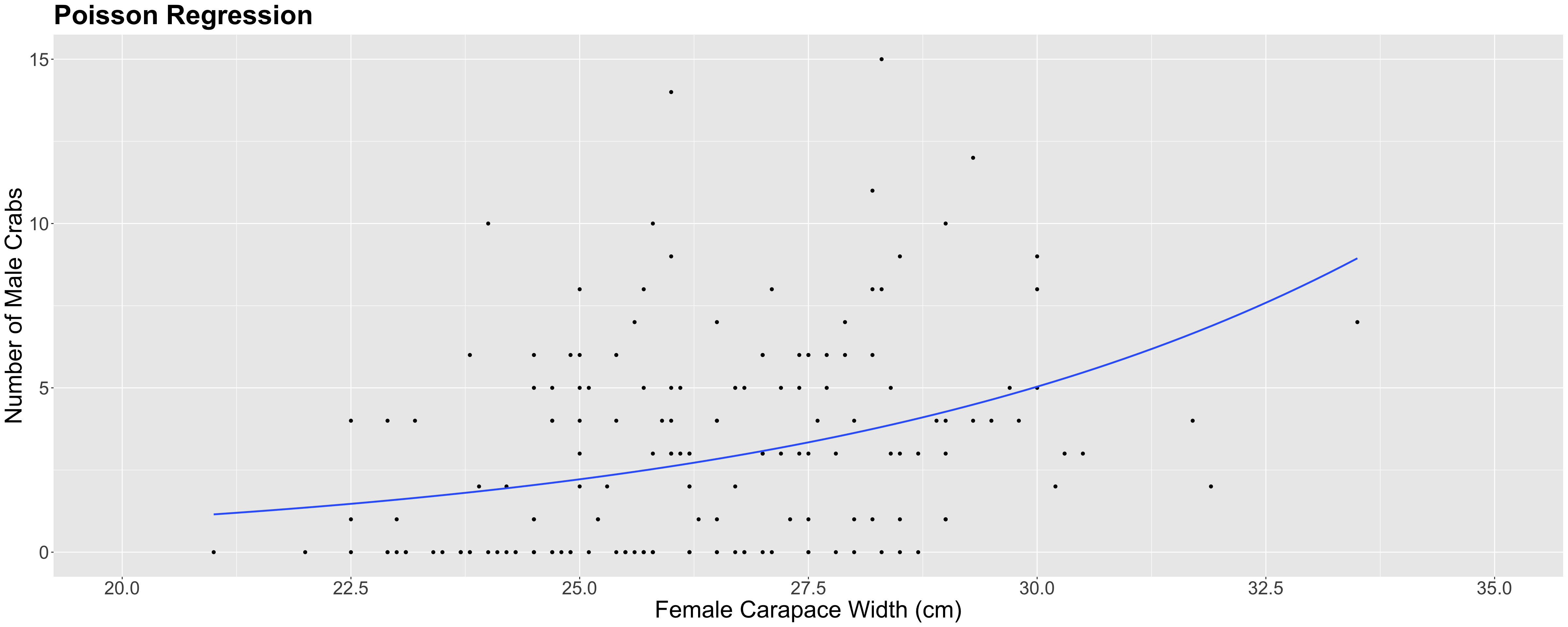
• Whether n_males and female carapace width are statistically associated and by how much.
• Whether n_males and female color of the prosoma are statistically associated and by how much.

4.2. Exploratory Data Analysis

iClicker Question

By checking the below plot, do you think n_males increases with the female carapace width?

A. Of course!

B. Not really.

C. I am pretty uncertain about an increasing or decreasing pattern.

Let us proceed with the data wrangling!

group_avg_width <- crabs|>
  mutate(intervals = cut(crabs$width, breaks = 10)) |>
  group_by(intervals) |>
  summarise(mean = mean(n_males), n = n()) 
group_avg_width

# A tibble: 10 × 3
   intervals    mean     n
   <fct>       <dbl> <int>
 1 (21,22.2]    0        2
 2 (22.2,23.5]  1       14
 3 (23.5,24.8]  1.77    26
 4 (24.8,26]    2.98    43
 5 (26,27.2]    2.53    32
 6 (27.2,28.5]  4.15    33
 7 (28.5,29.8]  4       13
 8 (29.8,31]    4.86     7
 9 (31,32.2]    3        2
10 (32.2,33.5]  7        1

Then, some plotting…

More plotting…

• Response n_males is count-type. So, a more appropriate standalone plot is a bar chart.
• Note the right-skewness.

4.3. Data Modelling Framework

• Poisson regression is the primary resource when it comes to modelling counts.
• This model also fits into the GLM class.

• A Poisson random variable refers to discrete data with non-negative integer values that count something.

These counts could happen during a given timeframe or even a space such as a geographic unit!

Distributional Insights

• A Poisson regression model assumes a random sample of \(n\) count observations \(Y_i\)s, hence independent (but not identically distributed!).

\[Y_i \sim \text{Poisson}(\lambda_i)\]

• Note \(\mathbb{E}(Y_i) = \lambda_i > 0\) and \(\text{Var}(Y_i) = \lambda_i > 0\).

Heads-up: Given that \(\mathbb{E}(Y_i) = \text{Var}(Y_i) = \lambda_i\), we also assume equidispersion. Furthermore, \(\lambda_i\) is continuous!

Going back to the crabs dataset…

• The events are the number of male crabs (n_males) around a space: the female breeding nest.

• Let \(X_{\texttt{width}_i}\) be the \(i\)th value for the regressor width in our dataset. We could use identity link function as in \[ h(\lambda_i) = \lambda_i = \beta_0 + \beta_1 X_{\texttt{width}_i}. \]

However…

• We have a response range issue!

• Instead, we will use the natural logarithm of the mean \(\log(\lambda_i)\).

• In the crabs dataset with width as a regressor, the model is depicted via this systematic component: \[ h(\lambda_i) = \log(\lambda_i) = \beta_0 + \beta_1 X_{\texttt{width}_i}. \]

• The random component is implicitly contained in \[Y_i \sim \text{Poisson}(\lambda_i).\]

4.4. Estimation

• Under a general framework with \(k\) regressors, the regression parameters \(\beta_0, \beta_1, \dots, \beta_k\) in the model are unknown.
• We will use glm() to get the estimates \(\hat{\beta}_0, \hat{\beta}_1, \dots \hat{\beta}_k\).
• These estimates are obtained through maximum likelihood where we assume a Poisson joint probability mass function of the \(n\) responses \(Y_i\).

4.5. Inference

• We can determine whether a regressor is statistically associated with the logarithm of the response’s mean through hypothesis testing for \(\beta_j\).
• We use \(\hat{\beta}_j\) and its standard error, \(\mbox{se}\left(\hat{\beta}_j\right)\).

• Then, we test the below hypotheses via the Wald statistic \(z _j= \frac{\hat{\beta}_j}{\mbox{se}(\hat{\beta}_j)}\) as in: \[\begin{align*} H_0: \beta_j &= 0 \\ H_a: \beta_j &\neq 0. \end{align*}\]

Solving one part of our initial inquiries!

Is female caparace width statistically associated to the logarithm of mean of the counts of satellite male crabs residing around a female crab nest?

• We have evidence to state that female carapace width is statistically associated to the logarithm of the mean of n_males.

Plotting our estimated regression function!

Is there a positive relationship between carapace width and the original scale of the response n_males?

4.6. Coefficient Interpretation

• Let us fit a second model with two regressors: width (\(X_{\texttt{width}_i}\)) and color (\(X_{\texttt{color_darker}_i}\), \(X_{\texttt{color_light}_i}\), and \(X_{\texttt{color_medium}_i}\)): \[ h(\lambda_i) = \log (\lambda_i) = \beta_0 + \beta_1 X_{\texttt{width}_i} + \beta_2 X_{\texttt{color_darker}_i} + \\ \beta_3 X_{\texttt{color_light}_i} + \beta_4 X_{\texttt{color_medium}_i}. \]

Using glm()and tidy()

Firstly…

• Let us focus on the coefficient corresponding to carapace width, while keeping color constant.
• Consider an observation with a given value \(X_{\texttt{width}} = \texttt{w}\) cm, then:

\[\begin{align*} \log \left( \lambda_{\texttt{width}} \right) &= \beta_0 + \beta_1 \overbrace{\texttt{w}}^{X_{\texttt{width}}} + \\ & \qquad \underbrace{\beta_2 X_{\texttt{color_darker}} + \beta_3 X_{\texttt{color_light}} + \beta_4 X_{\texttt{color_medium}}}_{\text{Constant}}. \end{align*}\]

Now…

• For another observation with a given \(X_{\texttt{width + 1}} = \texttt{w} + 1\) cm, we have that:

\[\begin{align*} \log \left( \lambda_{\texttt{width + 1}} \right) &= \beta_0 + \beta_1 \overbrace{\texttt{w} + 1}^{X_{\texttt{width + 1}}} + \\ & \qquad \underbrace{\beta_2 X_{\texttt{color_darker}} + \beta_3 X_{\texttt{color_light}} + \beta_4 X_{\texttt{color_medium}}}_{\text{Constant}}. \end{align*}\]

Playing around with the math!

• If we set up the difference \(\log \left( \lambda_{\texttt{width}} \right) - \log \left( \lambda_{\texttt{width + 1}} \right)\), along with some logarithm properties and exponentiation, we end up with the following expression: \[\frac{\lambda_{\texttt{width + 1}} }{\lambda_{\texttt{width}}} = e^{\beta_1}.\]

• This expression indicates that the response varies in a multiplicative way when increased 1 cm in carapace width.

Solving another part of our initial inquiries!

\(\frac{\hat{\lambda}_{\texttt{width + 1}} }{\hat{\lambda}_{\texttt{width}}} = e^{\hat{\beta}_1} = 1.16\) indicates the mean count of male crabs (n_males) around a female breeding nest increases by \(16\%\) when increasing the female carapace width by \(1\) cm, while keeping color constant.

Then…

• Consider two observations: one \(\lambda_{\texttt{D}}\) with dark color of the prosoma (the baseline) and another \(\lambda_{\texttt{L}}\) with light color:

\[\begin{align*} \log \left( \lambda_{\texttt{D}} \right) = \beta_0 + \overbrace{\beta_1 X_{\texttt{width}}}^{\text{Constant}} + \beta_2 \overbrace{X_{\texttt{color_darker}_{\texttt{D}}}}^0 + \\ \beta_3 \underbrace{X_{\texttt{color_light}_{\texttt{D}}}}_0 + \beta_4 \underbrace{X_{\texttt{color_medium}_{\texttt{D}}}}_0 \end{align*}\] \[\begin{align*} \log \left( \lambda_{\texttt{L}} \right) = \beta_0 + \overbrace{\beta_1 X_{\texttt{width}}}^{\text{Constant}} + \beta_2 \overbrace{X_{\texttt{color_darker}_{\texttt{L}}}}^0 + \\ \beta_3 \underbrace{X_{\texttt{color_light}_{\texttt{L}}}}_1 + \beta_4 \underbrace{X_{\texttt{color_medium}_{\texttt{L}}}}_0. \end{align*}\]

Playing around with the math!

• If we set up the difference \(\log \left( \lambda_{\texttt{L}} \right) - \log \left( \lambda_{\texttt{D}} \right)\), along with some logarithm properties and exponentiation, we end up with the following expression:

\[ \frac{\lambda_{\texttt{L}} }{\lambda_{\texttt{D}}} = e^{\beta_3}. \]

• This expression indicates that the response varies in a multiplicative way when the color of the prosoma changes from dark to light.

Solving another part of our initial inquiries!

\(\frac{\hat{\lambda}_{\texttt{L}} }{\hat{\lambda}_{\texttt{D}}} = e^{\hat{\beta}_3} = 1.55\) indicates that the mean count of male crabs (n_males) around a female breeding nest increases by \(55\%\) when the color of the prosoma changes from dark to light, while keeping the female carapace width constant.

4.7. Predictions

• Suppose we want to predict the mean count of male crabs (n_males) around a female breeding nest with a female carapace width of \(27.5\) cm and light color of the female prosoma.
• We could use the model poisson_model_2 as follows:

Interpretation

• The previous prediction can be interpreted in plain words as follows:

Given a female carapace width of \(27.5\) cm and light color of the female prosoma, we predict \(4.29\) male crabs around that female crab nest on average.

5. Overdispersion

• Population variances of some random variables could be a function of their respective means:
  • If \(X \sim \text{Exponential}(\lambda)\), then \(\mathbb{E}(X) = \lambda\) and \(\text{Var}(X) = \lambda^2\).
  • If \(X \sim \text{Binomial}(n , p)\), then \(\mathbb{E}(X) = n p\) and \(\text{Var}(X) = n p (1 - p)\).
  • If \(X \sim \text{Poisson}(\lambda)\), then \(\mathbb{E}(X) = \lambda\) and \(\text{Var}(X) = \lambda\).

How does equidispersion affect our Poisson regression model?

Heteroscedasticity

• We must clarify that GLMs naturally deal with some types of heteroscedasticity.
• For example, note that each observation \(i = 1, \dots, n\) in our training set (used to estimate a Poisson regression model) is assumed as: \[Y_i \sim \text{Poisson}(\lambda_i).\]

In many cases…

• The variance of our data is sometimes larger than the variance considered by our model as in the basic Poisson regression.

Heads-up: When the variance is larger than the mean in a random variable, we have overdispersion.

Going back to poisson_model_2!

• Let us go back to our poisson_model_2 with the log link function from the crabs dataset with two regressors: width (\(X_{\texttt{width}_i}\)) and color (\(X_{\texttt{color_darker}_i}\), \(X_{\texttt{color_light}_i}\), and \(X_{\texttt{color_medium}_i}\)) for the \(i\)th observation:

\[ \begin{align*} h(\lambda_i) &= \log (\lambda_i) = \beta_0 + \beta_1 X_{\texttt{width}_i} + \\ & \qquad \beta_2 X_{\texttt{color_darker}_i} + \beta_3 X_{\texttt{color_light}_i} + \beta_4 X_{\texttt{color_medium}_i}. \end{align*} \]

Testing for overdispersion!

• We will test whether there is overdispersion in this Poisson regression model via function dispersiontest(), (from package {AER}).
• Let \(Y_i\) be the \(i\)th Poisson response in the count regression model.

• Ideally in the presence of equidispersion, \(Y_i\) has the following parameters: \[\begin{gather*} \mathbb{E}(Y_i) = \lambda_i \\ \text{Var}(Y_i) = \lambda_i. \end{gather*}\]

Test Specifics

• The test uses the following mathematical expression: \[ \text{Var}(Y_i) = \overbrace{(1 + \gamma)}^\text{Dispersion Factor} \lambda_i, \]

• Moreover, we have the following hypotheses: \[\begin{gather*} H_0: 1 + \gamma = 1 \\ H_a: 1 + \gamma > 1. \end{gather*}\]
• When there is evidence of overdispersion in our data, we will reject \(H_0\) under a pre-specified significance level \(\alpha\).

Running the test on poisson_model_2

With \(\alpha = 0.05\), we reject \(H_0\) since the \(p\text{-value} < .001\). Hence, the poisson_model_2 has overdispersion.

• Therefore, what modelling alternative do we have?

6. Negative Binomial Regression

• Let \[Y_i \sim \text{Negative Binomial} (m, p_i) \quad \text{for} \quad i = 1, \dots, n.\]
• This distribution has the following mean and variance: \[\begin{gather*} \mathbb{E}(Y_i) = \frac{m(1 - p_i)}{p_i} \\ \text{Var}(Y_i) = \frac{m(1 - p_i)}{p_i^2} \end{gather*}\]

6.1. Reparametrization

• Let us reparametrize the previous mean and variance: \[\begin{equation*} \lambda_i = \frac{m (1 - p_i)}{p_i} \qquad \Rightarrow \qquad p_i = \frac{m}{m + \lambda_i}, \end{equation*}\]

• Hence:

\[\begin{gather*} \mathbb{E}(Y_i) = \lambda_i \\ \text{Var}(Y_i) = \lambda_i \left( 1 + \frac{\lambda_i}{m} \right). \end{gather*}\]

6.2. General Modelling Framework

• As in the case of Poisson regression, the Negative Binomial case is a GLM with the following link function: \[\begin{equation*} h(\lambda_i) = \log(\lambda_i) = \beta_0 + \beta_1 X_{i,1} + \dots + \beta_k X_{i,k}. \end{equation*}\]

• Let \(\theta = \frac{1}{m}\). Then, Negative Binomial regression will assume the following variance: \[\begin{align*} \text{Var}(Y_i) = \lambda_i \left( 1 + \frac{\lambda_i}{m} \right) = \lambda_i + \theta \lambda_i^2. \end{align*}\]

6.3. Estimation

• Via a training set of size \(n\) whose responses are independent counts \(Y_i\) (\(i = 1, \dots, n\)), we use maximum likelihood estimation to obtain \(\hat{\beta}_0, \hat{\beta}_1, \dots, \hat{\beta}_k, \hat{\theta}\).
• To fit a Negative Binomial regression via R, we can use the function glm.nb() from package {MASS}.

Checking summaries!

iClicker Question

• Under the context of this crab problem with overdispersion as assessed by the overdispersion test, suppose we use poisson_model_2 to perform inference on the response and regressors.
• What is the consequence of using these underestimated standard errors compared to the ones from negative_binomial_model?

A. We are more prone to commit Type I errors (i.e., rejecting \(H_a\) when in fact it is true).

B. We are more prone to commit Type I errors (i.e., rejecting \(H_0\) when in fact it is true).

C. We are more prone to commit Type II errors (i.e., rejecting \(H_a\) when in fact it is true).

D. We are more prone to commit Type II errors (i.e., rejecting \(H_0\) when in fact it is true).