Lecture 4

Linear Mixed-effects Models

(Please, sign in on iClicker)

Today’s Learning Goals

By the end of this lecture, you should be able to:

• Identify the model assumptions in a linear Mixed-effects model.

• Associate a term (or combination of terms) in a Mixed-effects model with the following quantities:

  • Fixed effect estimates.
  • Variances of the random effects.
  • Regression coefficients for each group and population.
  • Predictions on existing groups and a new group.

Today’s Learning Goals (cont’d)

• Fit a linear Mixed-effects model in R, and extract estimates of the above quantities.
• Identify the consequences of fitting a Mixed-effects linear regression model when there are groups, whether a slope parameter is pooled or fit separately per group.
• Explain the difference between the distributional assumption on the random effects and the fixed effects estimates’ sampling distribution.

Outline

1. Linear Fixed-effects Model
2. Linear Mixed-effects Model

1. Linear Fixed-effects Model

• Let us start with different modelling techniques you learned in DSCI 561.
• So far, we have been working with regression models fitted with a training set of \(n\) independent elements.
• Given a set of \(k\) regressors \(X_{i,j}\) and a continuous response \(Y_i\), we fit a model:

\[Y_i = \beta_0 + \beta_1 X_{i,1} + \beta_2 X_{i,2} + \ldots + \beta_k X_{i,k} + \varepsilon_{i} \; \; \; \; \text{for} \; i = 1, \ldots, n.\]

• Parameters \(\beta_0, \dots, \beta_k\) are called fixed effects.

1.1. Grunfeld’s Investment Dataset

• Consider the following example: to study how gross investment depends on the firm’s value and capital stock, Grunfeld (1958) collected data from eleven different American companies over the years 1935-1954.

The data frame Grunfeld, from package {AER}, contains 220 observations from a balanced panel of 11 sampled American firms from 1935 to 1954 (20 observations per firm). The dataset includes a continuous response investment subject to two explanatory variables, market_value and capital.

Data Summary

• Firstly, we will load the data which has the following variables (those continuous refer to millions of USD):

1. investment: the gross investment, a continuous response.
2. market_value: the firm’s market value, a continuous explanatory variable.
3. capital: stock of plant and equipment, a continuous explanatory variable.

4. firm: a nominal explanatory variable with eleven levels indicating the firm (General Motors, US Steel, General Electric, Chrysler, Atlantic Refining, IBM, Union Oil, Westinghouse, Goodyear, Diamond Match, and American Steel).
5. year: the year of the observation (it will not be used in our analysis).

Data in R!

iClicker Question

• What class of data hierarchy do you observe in this dataset? Do you expect any class of correlation within the data points? Think about each hierarchical level as a possible sampling pool.

A. Yes, we have a data hierarchy with one level: firm. Still, there will not be a correlation among subsets of data points.

B. Yes, we have a data hierarchy with one level: firm. Hence, there will be a correlation among subsets of data points.

C. There is no data hierarchy at all. All observations in the training set are independent.

D. Yes, we have a data hierarchy with two levels: firm (level 1) and the corresponding yearly observations (level 2). Hence, there will be a correlation among subsets of data points.

Main Statistical Inquiries

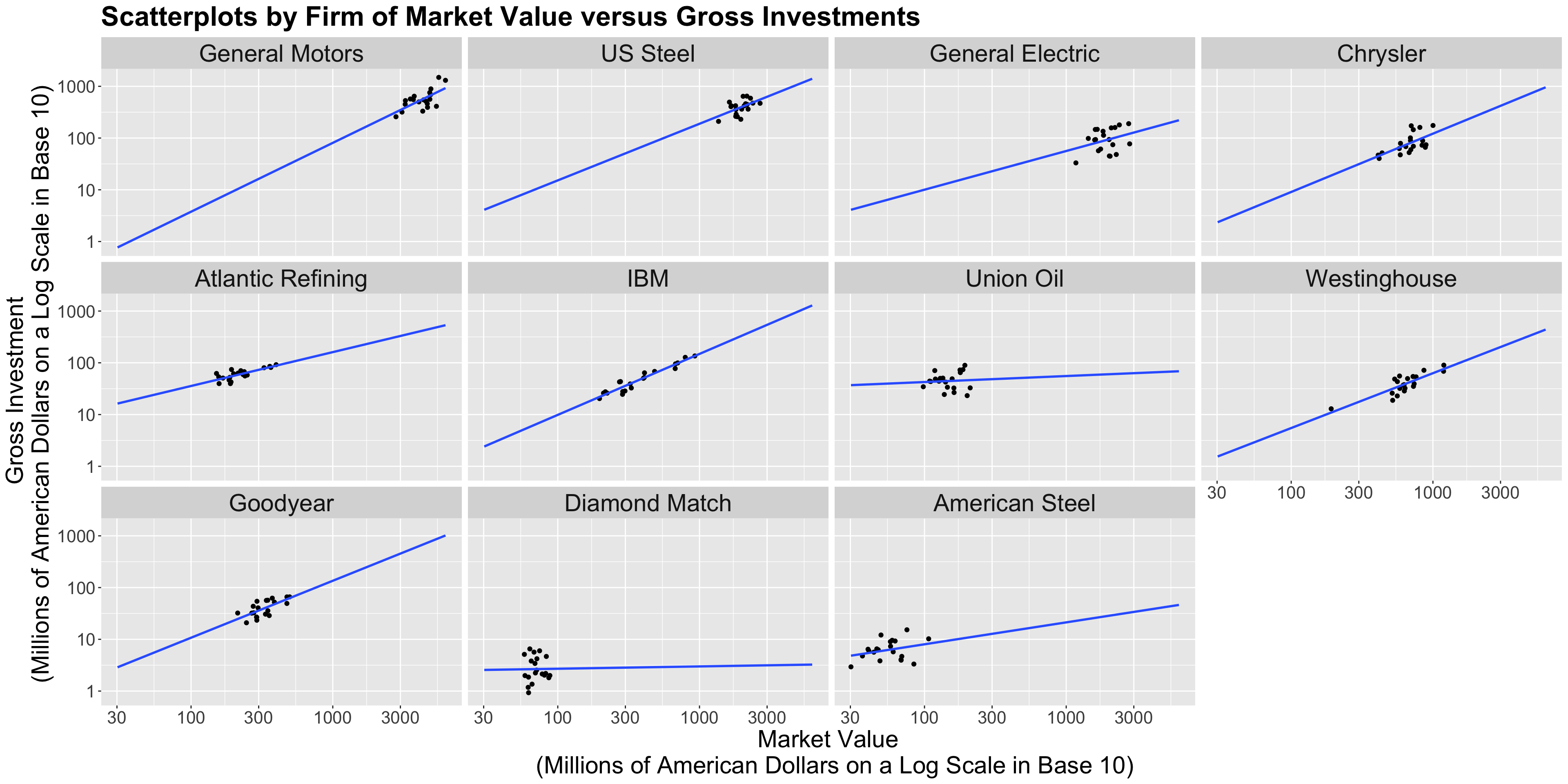
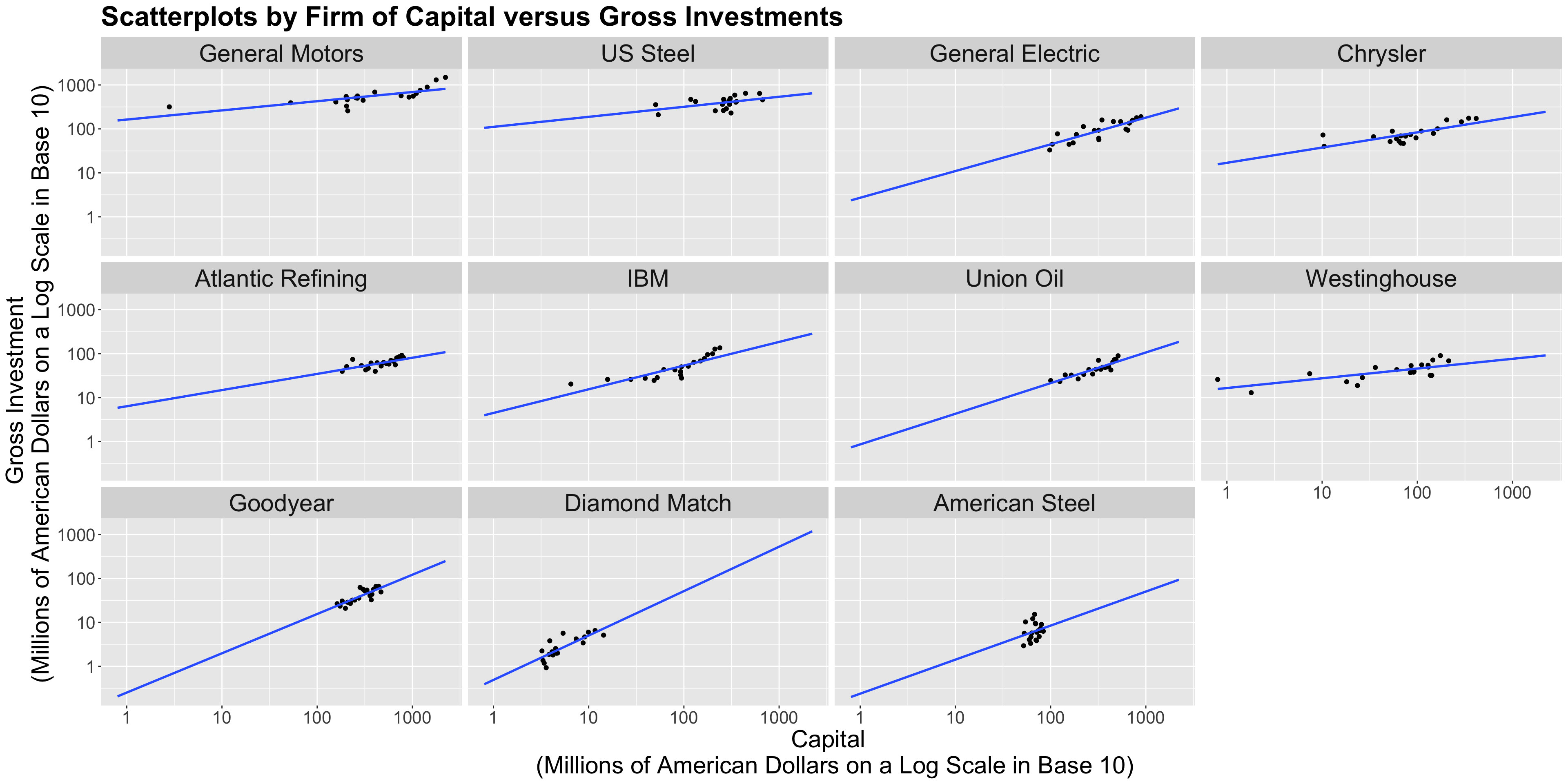
• We are interested in assessing the association of gross investment with market_value and capital in the population of American firms.
• Then, how can we fit a linear model to this data?

1.2. Exploratory Data Analysis

• Let us plot the 220 data points of investment versus market_value but facetted by firm and use geom_smooth() to fit sub-models by firm.

Heads-up: Only for plotting, we will transform both \(x\) and \(y\)-axes on the logarithmic scale in base 10 (trans = "log10"). This allows us to compare those firms under dissimilar market values, capital, and gross investments.

Plots!

More plots!

In-class Question

• What do you observe in the previous plots?

1.3. OLS General Modelling Framework

• Before digging into today’s new modelling approach, let us try a classical approach via Ordinary Least-squares (OLS) for comparative purposes.

Heads-up: Always keep in mind the main statistical inquiry when taking any given modelling approach.

1.3.1. Regression Alternatives

• Based on what we have seen via OLS in DSCI 561, there might be four possible approaches:

1. Take the average for each firm, and fit an ordinary least-squares (OLS) regression on the averages. This is not an ideal approach.
2. We could ignore firm. This is not an ideal approach.
3. Allow different intercepts for each firm.
4. Allow a different slope and intercept for each firm (i.e., an interaction model!).

1.3.2. OLS Ignoring Firm

• Let us start with this basic OLS model to warm up our modelling skills regarding setting up equations.
• The regression equation for the \(i\)th sampled observation will be:

\[\begin{align*} \texttt{investment}_{i} &= \beta_0 + \beta_1 \texttt{marketValue}_{i} + \beta_2\texttt{capital}_{i} + \varepsilon_{i} \\ & \qquad \qquad \qquad \qquad \qquad \qquad \text{for} \; i = 1, \ldots, 220. \end{align*}\]

Code in R!

1.3.3. OLS Regression with Varying Intercept

• Let us estimate another OLS model with investment as a response to market_value and capital as regressors but with varying intercepts by each firm.
• We can use lm() by adding - 1 on the right-hand side of the argument formula.
• This - 1 will allow the baseline firm to have its intercept (i.e., renaming (Intercept) in column estimate with firmCompanyName).

Fitting model in R!

Glancing model in R!

Model Comparison

• By checking the adj.r.squared, we see that model_varying_intercept has a larger value (0.959) than ordinary_model (0.816).
• Note that model_varying_intercept is equivalent to just fitting the OLS model using:

formula = investment ~ market_value + capital + firm.

• Let us check the above fact!

Using lm() without -1

\(F\)-test

• Going back to model_varying_intercept and ordinary_model, we can test if there is a gain in considering a varying intercept versus fixed intercept.
• Hence, we will make a formal \(F\)-test to check whether the model_varying_intercept fits the data better than the ordinary_model.

Testing Conclusion

• We obtain a \(p\text{-value} < .001\).
• Thus, with \(\alpha = 0.05\), we have evidence to conclude that model_varying_intercept fits the data better than the ordinary_model.

• However, this costs us one extra degree of freedom per firm except for the baseline.
• Therefore, we lose another 10 degrees of freedom (column DF in the anova() output).

Heads-up: In this specific case, losing 10 degrees of freedom is not a big deal with 220 data points. Nonetheless, when data is scarce or the model’s complexity demands a large amount of regression parameters, this could be an issue.

iClicker Question

• What is the sample’s regression equation for model_varying_intercept?

A. \[\begin{align*} \texttt{investment}_{i,j} &= \beta_{0} + \beta_1 \texttt{marketValue}_{i,j} + \beta_2\texttt{capital}_{i,j} + \varepsilon_{i,j} \\ & \qquad \qquad \quad \text{for} \; i = 1, \ldots, 20 \; \; \text{and} \; \; j = 1, \ldots, 11. \end{align*}\]

B. \[\begin{align*} \texttt{investment}_{i} &= \beta_{0} + \beta_1 \texttt{marketValue}_{i} + \beta_2\texttt{capital}_{i} + \varepsilon_{i} \\ & \qquad \qquad \quad \text{for} \; i = 1, \ldots, 220. \end{align*}\]

C. \[\begin{align*} \texttt{investment}_{i,j} &= \beta_{0,j} + \beta_1 \texttt{marketValue}_{i,j} + \beta_2\texttt{capital}_{i,j} + \varepsilon_{i,j} \\ & \qquad \qquad \quad \text{for} \; i = 1, \ldots, 20 \; \; \text{and} \; \; j = 1, \ldots, 11. \end{align*}\]

1.3.4. OLS Regression for Each Firm

• We fit a more complex OLS model with two interactions.

Glancing model in R!

A note on this model!

• In this case, we are fitting eleven linear regressions, each with 20 points.

Heads-up: We have plenty of data points in this case for all the degrees of freedom required to estimate each parameter. Nonetheless, this might not hold for other small datasets. Also, we must consider other modelling scenarios in which there may be more than two regressors of interest with different natures (discrete and continuous), which may require a large number of degrees of freedom.

iClicker Question

What is the sample’s regression equation for model_by_firm?

A.

\[\begin{align*} \texttt{investment}_{i,j} &= \beta_{0,j} + \beta_{1,j} \texttt{marketValue}_{i,j} + \beta_{2,j} \texttt{capital}_{i,j} + \varepsilon_{i,j} \\ & \qquad \qquad \quad \text{for} \; i = 1, \ldots, 20 \; \; \text{and} \; \; j = 1, \ldots, 11. \end{align*}\]

B.

\[\begin{align*} \texttt{investment}_{j} &= \beta_{0} + \beta_1 \texttt{marketValue}_{j} + \beta_2\texttt{capital}_{j} + \varepsilon_{j} \\ & \qquad \qquad \quad \text{for} \; j = 1, \ldots, 11. \end{align*}\]

C. \[\begin{align*} \texttt{investment}_{i,j} &= \beta_{0,i} + \beta_{1,i} \texttt{marketValue}_{i,j} + \beta_{2,i} \texttt{capital}_{i,j} + \varepsilon_{i,j} \\ & \qquad \qquad \quad \text{for} \; i = 1, \ldots, 20 \; \; \text{and} \; \; j = 1, \ldots, 11. \end{align*}\]

How to interpret the coefficients in this model?

Each regression coefficient is associated with a firm. For example, \(\texttt{firmUS Steel:capital} = 0.02\) means that the variable capital has a slope of \(0.02 + 0.37 = 0.39\) for US Steel. We can double-check this by estimating an individual linear regression for US Steel.

In-class Question

• Now, after all these OLS modelling approaches, are we in line with the main modelling objective with all these linear regression models?

2. Linear Mixed-effects Model

• Let us take a step back and think about a population of companies. For instance, all American companies.

• Grunfeld did not collect data on all the American companies but sampled 11 companies from this population. The author was interested in assessing whether market_value and capital were related to investment and by how much.

Mixed Intercept!

• Let us assume that the \(j\)th sampled firm has its own intercept \(b_{0,j}\) and the overall fixed intercept is \(\beta_0\) for all American companies.
• Therefore, for the \(j\)th firm we define the following mixed intercept:

\[\begin{equation*} \beta_{0,j} = \beta_0 + b_{0,j}. \end{equation*}\]

• Term \(b_{0,j}\) will change due to chance since it is linked the \(j\)th sampled firm which would make it a random effect.

Changing our Regression Paradigm!

• The regression paradigm of estimating a fixed unknown intercept \(\beta_0\) will change now. Moreover, the intercept \(\beta_{0,j}\) is what we call a mixed effect.

\[\begin{align*} \texttt{investment}_{i,j} &= \overbrace{\beta_{0,j}}^{\text{Mixed Effect}} + \beta_1 \texttt{marketValue}_{i,j} + \\ & \qquad \quad \beta_2\texttt{capital}_{i,j} + \varepsilon_{i,j} \\ &= (\beta_0 + b_{0,j}) + \beta_1 \texttt{marketValue}_{i,j} + \\ & \qquad \quad \beta_2\texttt{capital}_{i,j} + \varepsilon_{i,j} \\ & \qquad \qquad \; \; \; \; \text{for} \; i = 1, \ldots, n_j \; \; \text{and} \; \; j = 1, \ldots, 11. \end{align*}\]

Heads-up: Note that \(n_j\) is making the model even more flexible by allowing different numbers of observations \(n_j\) in each \(j\)th firm.

Now…

\[b_{0,j}\sim \mathcal{N}(0, \sigma_0^2)\]

is called a random effect and we assume it is independent of the error component

\[\varepsilon_{i,j}\sim \mathcal{N}(0, \sigma^2).\]

Heads-up: The observations for the same firm (group) share the same random effect making a correlation structure.

And the variance is…

• The variance of the \(i\)th response for the \(j\)th firm will be \[\begin{equation*} \text{Var}(\texttt{investment}_{i,j}) = Var(b_{0,j}) + Var(\varepsilon_{i,j}) = \sigma_0^2 + \sigma^2. \end{equation*}\]

• For the \(k\)th and \(l\)th responses, within the \(j\)th firm, the correlation is given by: \[\begin{equation*} \text{Corr}(\texttt{investment}_{k,j}, \texttt{investment}_{l,j}) = \frac{\sigma^2_0}{\sigma_0^2 + \sigma^2}. \end{equation*}\]

Random Slopes!

• We could even go further and model random slopes, along with the existing fixed ones, as follows: \[\begin{align*} \texttt{investment}_{i,j} &= \overbrace{\beta_{0,j}}^{\text{Mixed Effect}} + \overbrace{\beta_{1,j}}^{\text{Mixed Effect}} \times \texttt{marketValue}_{i,j} + \\ & \qquad \quad \overbrace{\beta_{2,j}}^{\text{Mixed Effect}} \times \texttt{capital}_{i,j} + \varepsilon_{i,j} \\ &= (\beta_0 + b_{0,j}) + (\beta_1 + b_{1,j}) \times \texttt{marketValue}_{i,j} + \\ & \qquad \quad (\beta_2 + b_{2,j}) \times \texttt{capital}_{i,j} + \varepsilon_{i,j} \\ & \qquad \qquad \qquad \text{for} \; i = 1, \ldots, n_j \; \; \text{and} \; \; j = 1, \ldots, 11; \end{align*}\]

• Note \((b_{0,j}, b_{1,j}, b_{2,j})^{T} \sim \mathcal{N}_3(\mathbf{0}, \mathbf{D})\), where \(\mathbf{0} = (0, 0, 0)^T\) and \(\mathbf{D}\) is a generic covariance matrix.

2.1. What is this Generic Covariance Matrix \(\mathbf{D}\)?

• This is a standard form in linear mixed effects modelling.
• Hence, this matrix becomes:

\[\begin{equation*} \mathbf{D} = \begin{bmatrix} \sigma_{0}^2 & \rho_{01} \sigma_{0} \sigma_{1} & \rho_{02} \sigma_{0} \sigma_{2}\\ \rho_{01} \sigma_{0} \sigma_{1} & \sigma_{1}^2 & \rho_{12} \sigma_{1} \sigma_{2}\\ \rho_{02} \sigma_{0} \sigma_{2} & \rho_{12} \sigma_{1} \sigma_{2} & \sigma_{2}^2 \end{bmatrix} = \begin{bmatrix} \sigma_{0}^2 & \sigma_{0, 1} & \sigma_{0, 2} \\ \sigma_{0, 1} & \sigma_{1}^2 & \sigma_{1,2}\\ \sigma_{0, 2} & \sigma_{1, 2} & \sigma_{2}^2 \end{bmatrix} \end{equation*}\]

Important Notes

• The joint Normal distribution explains the variability of random regression coefficients and intercepts. The spread does not change when we collect more data.
• The sampling distribution explains the uncertainty in the fixed regression estimates and gets narrower as we collect more data.

2.2. Model Fitting, Inference, and Coefficient Interpretation

• Let us estimate the regression model with a mixed intercept only (mixed_intercept_model) via the function lmer() from package lme4.
• Note that (1 | firm) allows the model to have a random intercept by firm.

Estimate the Mixed-effects

• Now, let us estimate the Mixed-effects regression model with mixed intercept and slopes (full_mixed_model).

Inference

• Let us proceed with inference using mixed_intercept_model.
• We now assess whether the fixed effects are statistically associated with investment in each model via summary().
• We will use the package lmerTest via function summary().

Inferential Conclusion

• We can see that market_value and capital are significant with \(\alpha = 0.05\) in both models.
• Moreover, the regression coefficients’ interpretation for the fixed effects will be on the effect these regressors have on the population investment mean of the American companies.
• We can obtain the estimated coefficients by firm along with the intercepts for both models via coef().

Getting coefficients in R!

Some notes!

• Column (Intercept) is the sum \(\hat{\beta}_0 + \hat{b}_{0,j}\).
• Note the estimated regression coefficients for market_value and capital are the same since mixed_intercept_model only has \(\beta_1\) and \(\beta_2\) as its general modelling setup.

• The coefficient summary changes in full_mixed_model given that we also include random effects for market_value and capital.
• Columns market_value and capital are the sums \(\hat{\beta}_1 + \hat{b}_{1,j}\) and \(\hat{\beta}_2 + \hat{b}_{2,j}\), respectively.
• Column (Intercept) is the sum \(\hat{\beta}_0 + \hat{b}_{0,j}\).

In-class Question

• Note the standard errors for the estimated slopes in market_value and capital behave in a really particular way when comparing the OLS model_varying_intercept and the Mixed-effects full_mixed_model.
• Therefore, what are the advantages of a Mixed-effects model over an OLS model with fixed-effects only?

2.3. Estimation

• Mixed-effects models are still fit using likelihood ideas.
• Compared to OLS, there is more to estimate:
  • Fixed effects: intercept and coefficients.
  • Overall variance: \(\sigma^2\).
  • Variance components (associated to random effects): how much groups/subjects vary (and sometimes how random effects move together).

REML: Restricted Maximum Likelihood

• REML is a common estimation approach for Mixed-effects regression.

• Intuition: estimating fixed effects “uses up” information, so plain maximum likelihood estimation (MLE) can underestimate random-effect variances.
• REML focuses on variation left over after accounting for fixed effects.

Two Steps in Practice

1. Estimate variance components (random-effect variances/covariances and \(\sigma^2\)).
2. Estimate fixed effects given those variance estimates (a weighted regression accounting for within-group correlation).

2.4. Prediction

We can make two classes of predictions with Mixed-effects models:

1. To predict on an existing group, we find that group’s regression coefficients (and therefore model function) by summing the fixed effects and (if present) the random effects, then use that model function to make predictions.

2. To predict on a new group (using a mean prediction), we use the fixed effects as the regression coefficients (because the random effects have mean zero) and use that model function to make predictions.

Code in R!

• For predictions on an existing group in our training set we have:

If we wanted to predict the investment for General Motors with a market_value of USD \(\$2,000\) million and capital of USD \(\$1,000\) million, then our answer would be USD \(\$537.4\) million.

• This prediction uses \(\hat{\beta}_0\), \(\hat{\beta}_1\), \(\hat{\beta}_2\), \(\hat{b}_{0, j}\), \(\hat{b}_{1, j}\), and \(\hat{b}_{2, j}\).

Make prediction for new observations!

• For predictions on American companies in general, we have:

If we wanted to predict the MEAN investment for American companies with a market_value of USD \(\$2,000\) million and capital of USD \(\$1,000\) million, then our answer would be USD \(\$341.51\) million. This prediction only uses \(\hat{\beta_0}\), \(\hat{\beta_1}\), and \(\hat{\beta_2}\).

3. Wrapping Up

• In many different cases, when there is a correlation structure in our observations, OLS models are not suitable for our inferential or predictive inquiries.
• Therefore, linear Mixed-effects models are suitable for correlated observations.
• Nonetheless, the model’s complexity will also be in function of our specific inquiries.
• We can even extend the Mixed-effects approach to generalized linear models (GLMs)!