Lecture 5

Survival Analysis

(Please, sign in on iClicker)

Today’s Learning Goals

By the end of this lecture, you should be able to:

• Identify when data is censored.
• Understand the consequence of subsetting to uncensored data or ignoring the censored property instead of using Survival Analysis methods.
• Obtain univariate estimates for the mean, median, and survival function in R with a parametric technique.

Today’s Learning Goals (cont’d)

• Obtain univariate estimates for the mean, median, and survival function in R with the Kaplan-Meier technique.
• Identify when the Kaplan-Meier survival function estimate cannot produce mean and high quantile estimates.

Today’s Learning Goals (cont’d)

• Outline the modelling framework of a Cox Proportional Hazards model.
• Fit a Cox Proportional Hazards model in R.
• Interpret the regression coefficients of a Cox Proportional Hazards model, and identify the model assumptions.
• Obtain predicted survival functions from a Cox Proportional Hazards model.

Outline

0. What have we covered so far?
1. Time to Event and Censoring
2. Censoring Examples
3. Key Concepts
4. Estimating the Survival Function
5. Cox Proportional Hazards Model

0. What have we covered so far?

• In terms of a conditioned mean response on its respective regressors, the classical Ordinary Least-squares (OLS) model is not enough when we encounter the following:
  1. Restricted continuous response range.
  2. Discrete responses.

And…

• Discrete responses need a different approach, i.e., generalized linear models (GLMs) via different link functions as follows:
  • Binary Logistic regression for binary responses.
  • Poisson or Negative Binominal regressions for count-type responses.
  • Multinomial Logistic regression for categorical and nominal responses.
  • Ordinal Logistic regression for categorical and ordinal responses.

Furthermore

• We can extend the OLS and GLM approaches to a mixed-effects framework. Therefore, we will be able to incorporate complex correlated data structures in our training sets.

• However, what happens when we encounter censored data in a continuous response framework?

A new class of data!

• Let us dig into this new class of data we have not seen so far.
• Modelling survival times can involve three statistical approaches: parametric, semiparametric, and non-parametric.

1. Time to Event and Censoring

• Suppose that we want to analyze the time until an event occurs.
• For example:
  • The time until some equipment breaks.
  • The time that unemployed people will take to land a new job.

Heads-up!

• Although this field in Statistics is usually referred to as Survival Analysis, the event in question does not need to be related to actual “survival.”

The important thing is to understand that we are interested in the time until something happens.

In-class Question

• Nevertheless, why is this different? Cannot we just use the techniques we have learned so far (e.g., a Binary Logistic regression model)?

Now…

• What are the implications of not taking into account censoring in data?

• Removing censored data will result in estimate uncertainty to be larger than it could be if we were to include the censored data.

• Removing censored data could also result in biased estimates if data have only been collected for a short time.

2. Censoring Examples

2.1. Constant Right-censoring

• Suppose we want to study the time until patients with a specific type of cancer die.
• The study will be funded for ten years, i.e., after the 10th year, the study will end.
• So, we will only observe the exact time some patients died within ten years.
• If an individual did not die due to cancer at the end of the study, then all we know is that the time of occurrence for that individual is higher than ten years. We do not know the exact time that person will die from cancer.

Graphical representation!

2.2. Random Right-censoring

• We can have other types of censoring as well.

• Using the previous example, if a patient were hit by a bus and died in the accident, the death would be unrelated to cancer. Hence, all we know is that the patient did not die due to cancer until that moment.

• Or, in a less “dark” example, what if a patient you were following moves out of the country? It is an analogous situation.
• All we know is that the patient was alive until they moved.

What is the difference between constant and random right-censoring?

• The most significant difference is that we could have a single and constant censoring time point, or a non-defined random censoring time point.

• However, as long as the censoring is independent of the time of the event of interest, we can deal with both situations quite similarly.

• There are other types of censoring besides right-censoring, but right-censoring is the most common one, and it will be the focus of this lecture.

2.3. Left-Censoring

• Suppose you want to know when kids learn how to ski.
• One of the kids participating in your study already knows how to ski. So, the event already happened in a past time, but you cannot know precisely when it was.
• All you know is that it was before the current time.

3. Key Concepts

• We learned in DSCI 551 that a random variable is characterized by its probability distribution (either density if continuous, or mass if discrete).
• In Survival Analysis, however, we frequently do not try to model the distribution directly. Instead, the focus is on modelling the survival or hazard functions.

Survival and Hazard Functions

• These two functions are quite crucial in Survival Analysis because they have special interpretations.
• If we know either of them, we can obtain the probability distribution for the time until an event occurs.
• They are just alternative ways to represent a probability distribution.

3.1. Survival Function

• For this function, let us consider a continuous random variable

\[Y = \text{Time when an event of interest occurs.}\]

• We know that the cumulative distribution function (CDF) of \(Y\) tells us the probability that the event of interest occurs before a certain point in time \(t\):

\[ F_Y(t) = P(Y \leq t). \]

Probability of an Event

• However, as the name suggests, in Survival Analysis, we are more interested in the probability that the event WILL NOT occur before a certain point in time \(t\) (i.e., the subject survives at least at point \(t\)):

\[ S_Y(t) = P(Y > t) = 1 - F_Y(t). \]

• \(S_Y(t)\) is called the survival function.

For example…

• Suppose that \(Y\) is being measured in days. So, we can measure the probability that the event of interest will not occur before \(t = 10\) days by

\[ S_Y(10) = P(Y > 10) = 1 - F_Y(10). \]

• Furthermore, as we can see in the next plot, note that any survival function (measured as a probability on the \(y\)-axis with time on the \(x\)-axis) WILL ALWAYS be monotonically decreasing as time goes by.

An example of survival function!

Source: Kleinbaum and Klein (2005).

Is the Survival Function Enough?

• Note that the survival function \(S_Y(t)\) fully characterizes \(Y\). In other words, if we know the survival function, we have everything we need about \(Y\).
• For instance, we can get the CDF \(F_Y(t)\) as follows: \[ F_Y(t) = 1 - S_Y(t). \]

• We could also get the probability density function (PDF): \[\begin{align*} f_Y(t) = \frac{dF_Y(t)}{dt} = -\frac{dS_Y(t)}{dt}. \end{align*}\]

3.2. Hazard Function

• The hazard function \(\lambda(t)\), the instantaneous rate of event occurrence per unit of time, is given by

\[ \lambda(t) = \lim_{\Delta t\rightarrow 0} \frac{P(t\leq Y < t+\Delta t | Y\geq t)}{\Delta t} = \frac{f_Y(t)}{S_Y(t)}. \]

Heads-up: One can interpret \(\lambda(t)\Delta t\) as the approximate probability of the event occurring immediately, given that the event has not occurred up until time \(t\).

Example

• Since we know how to calculate the survival function \(S_Y(t)\) from the cumulative distribution \(F_Y(t)\), we can obtain the survival function for any positive random variable.

Why positive?

• Because it measures the time until the event happens, and time cannot be negative in this context.
• Let us check an example of the Weibull distribution case to model \(S_Y(t)\).

The Weibull Case

• The Weibull distribution is one of the most popular parametric modelling choices in Survival Analysis to model \(S_Y(t)\).
• Let \[Y \sim \text{Weibull}(\alpha, \beta).\]

• Its PDF is given by: \[ f_Y(t) = \frac{\alpha}{\beta^\alpha}t^{\alpha - 1}\exp\left[-\left(\frac{t}{\beta}\right)^{\alpha}\right] \quad \text{for} \quad t, \alpha, \beta > 0. \]
• Note \(\alpha\) is called the shape parameter and \(\beta\) is the scale parameter.

Some notes

• If \(\alpha = 1\) we get the exponential distribution with parameter \(\beta\).
• Generally speaking, the terms shape and scale along with location, are broadly used in statistical distributions for the following:

• Location: A parameter of this class shifts the distribution of interest to the left or right of the \(x\)-axis.
• Scale: A parameter of this class stretches out (if it is large) of squeezes (if it is small) the distribution of interest.
• Shape: This parameter is more tricky to define since it affects the form of the distribution rather than just stretching out or squeezing.

Weibull’s CDF and Survival Functions

• Weibull’s CDF is given by

\[ F_Y(t) = 1 - \exp\left[-\left(\frac{t}{\beta}\right)^{\alpha}\right] \quad \text{for} \quad t > 0. \]

• Therefore, the survival function of the Weibull distribution is: \[ S_Y(t) = \exp\left[-\left(\frac{t}{\beta}\right)^{\alpha}\right] \quad \text{for} \quad t > 0. \]
• Now let us check how the survival function behaves under different scale and shape parameters.

Plots!

iClicker Question

• Suppose that the previous curves are the survival functions of cancer patients for different types of cancer.
• Interpret the Type D in comparison to the Type A and select the correct option below.

A. Type A is a more agressive type of cancer than Type D.

B. Both types of cancer are equally agressive.

C. Type D is a more agressive type of cancer than Type A.

Now…

• The hazard function for the Weibull distribution is given by: \[ \lambda(t) = \frac{f_Y(t)}{S_Y(t)} = \frac{\alpha}{\beta^\alpha}t^{\alpha - 1}. \]

iClicker Question

• What happens if \(\alpha = 1\)? Select the correct option below.

A. The Weibull’s hazard function increases over time.

B. The Weibull’s hazard function is constant (does not depend on the time).

C. The Weibull’s hazard function decreases over time.

Plots!

In-class Question

• Suppose that these curves are the hazard functions of cancer patients for different types of cancer.
• Let us compare the blue (Type D) and green (Type A) curves.

Note

• Other heavy-tailed distributions can also be used to model the survival function, such as:

  • Log-normal.
  • Generalized Gamma.
  • Rayleigh.
  • Pareto.

4. Estimating the Survival Function

• We will not know the probability distribution to be used in our survival and hazard functions in practice.
• We will only have a dataset from which we are interested in the survival time.

• It is up to you to make modelling decisions before estimating the corresponding survival parameter (in the case of a parametric approach).
• Moreover, there is also a quite popular non-parametric approach.

4.1. The Ovarian Dataset

• For this section, we will use the dataset ovarian from the package {survival}.

The ovarian dataset contains 26 survival records of a randomized trial that compares two (\(k = 2\)) treatments for ovarian cancer.

• We will use the following columns:
  • futime: The continuous survival or censoring time in days.
  • fustat: A binary factor indicating if the patient died (1 if true and 0 otherwise).
  • rx: A binary factor indicating the treatment group (1 or 2).

Data in R!

Main Statistical Inquiries

• We are interested in the following:

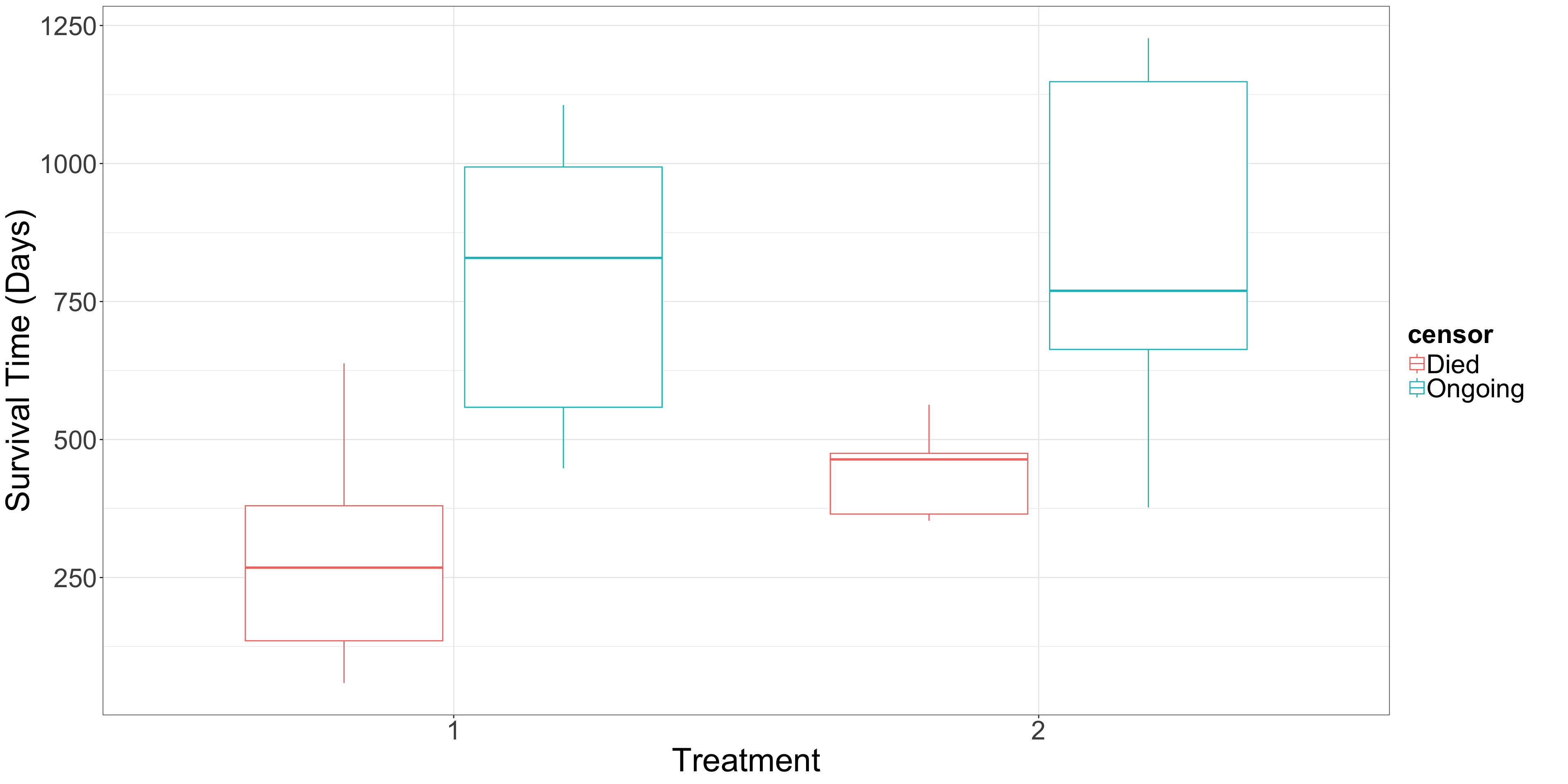
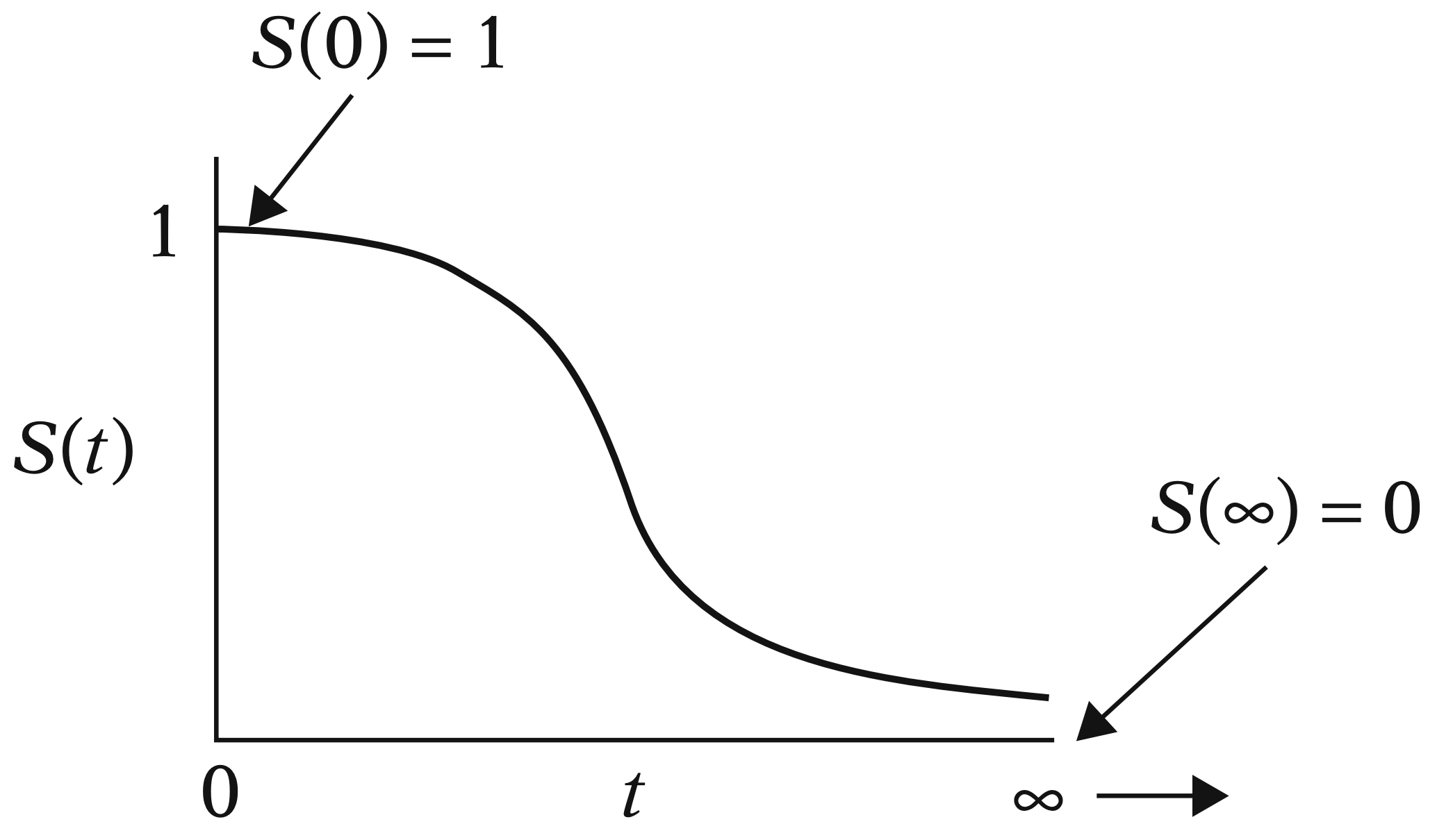
1. Regardless of the cancer treatment used, is it possible to estimate the overall survival function for this population of cancer patients?
2. Now, in terms of the specific cancer treatments, is there a statistical difference between both treatments? If so, can we quantify it? How would this be possible? Moreover, can we obtain the corresponding estimated survival functions per cancer treatment?

4.2. The Surv Function

• One of the key functions of the {survival} package is Surv() which receives two parameters.
  • The first one is the survival or censoring time, and the second one if the recorded time was censored (0) or whether the actual event happened (1).
  • The plus signs mean the futime was censored (we only know that the time is higher than that!).

What would happen if we discard the censored observations?

• This would be a serious mistake.
• In this case, we will probably underestimate the mean survival time because we are only considering the people that already died before the study ended.
• Let us compute the mean survival time for those non-censored observations.

Mean Time!

• Now, let us compute the mean time using all observations.

• By looking at these two figures, it seems there are problems with ignoring censored data. What should we do then?

Options

• There are two options for estimating quantities by incorporating the partial information contained in censored observations in the form of an estimated survival function of the population of interest:
  • Non-parametric.
  • Parametric.

Non-parametric

• If we do not make any distributional assumption, the Kaplan-Meier (KM) method can be used to estimate the survival function.
• This option will implicate the following:
  • RESTRICTED mean: it can be estimated as the area under an estimate of the survival function. Mathematically, this can be proved via integrals.
  • Quantiles: they can be estimated by inverting an estimate of the survival function.

Parametric

• If a distributional assumption is made, we can use censored likelihood-based methods to estimate the parameters of the chosen heavy-tailed PDF for the observed survival times (e.g., Weibull).

4.3. Non-parametric Estimation and Inference of the Survival Function with Kaplan-Meier

• Non-parametric estimation is handy when we have a training dataset of survival times, but we have no idea how the survival function looks!
• Furthermore, we want to err on the side of caution by no assuming any random variable distribution.

• KM is a non-parametric method to estimate the survival function. Its estimated survival curve has the form of a step function computed with conditional probabilities.
• This method is incredibly popular, and it is one of the most cited papers in Statistics (over 68,000 citations!). You can find the original 1958 paper here.

Estimation

• Since the survival function fully characterizes the random variable, if we know the survival function, we can estimate different statistics such as the mean, quantiles, etc.
• Let us estimate the survival function, obtain the mean survival time, and compare it with the two mean estimates we previously obtained: the mean survival time for those non-censored observations (\(351\) days) and the mean time of all observations (\(600\) days).

KM Estimation

• The KM estimate of the survival function can be obtained with survfit() from the package {survival}.
• It expects a formula, but we are still working with the null model (i.e., we consider all observations by not subsetting them by rx in the dataset ovarian).

Code in R!

• The KM estimate of the survival function can be obtained with survfit() from the package {survival}.
• It expects a formula, but we are still working with the null model (i.e., we consider all observations by not subsetting them by rx in the dataset ovarian).

Tidying the output!

Plotting via autoplot()

• To plot fit_km we can use autoplot() from package ggfortify for a ggplot2 style. Notice the “notches” where there is a censored observation.

KM Survival Function Estimate

Mean Survival Time

• Now that we have our estimated survival function, we could calculate the mean survival time and compare it with our previous “raw” mean estimates:
  • the mean survival time for those non-censored observations (\(351\) days), and
  • the mean time of all observations (\(600\) days).

• The r in rmean means restricted. Why restricted?

Because…

• The Kaplan-Meier estimate of the survival function does not always drop to zero (when the largest observation is censored).
• A common “fix” is to force the survival function to drop to zero at the largest observation. The mean estimate that results is called the restricted mean.

Median Survival Time

• We can find the median survival time on the printout of glance(fit_km).
• However, in general, we can use the quantile() S3 generic function from the package survival.

4.4. Parametric Estimation and Inference of the Survival Function with a Distributional Assumption

• As we discussed in the Weibull example above, if we know the distribution family of the survival time \(Y\), we can get its survival function of \[S_Y(t) = 1 - F_Y(t).\]
• Nonetheless, just knowing the family is not enough. What else do we need?

We need…

• The corresponding parameters of the distribution.
• If we assume that the data follows a specific distribution, say Weibull, all there is left for us to do is estimate the parameters of the Weibull.
• Nevertheless, we need to consider the censored data.
• We can do this using the survreg() function.

The survreg() Function

• Now, it is time to work with the survreg() function.
• This function corresponds to a parametric regression for a Survival Model.
• We will try another distribution. Let us fit the Log-normal distribution under one survival null regression model using dataset ovarian.

Comparing In-sample Fitted Values

• Now, let us compute the in-sample fitted values for both models.
• These fitted lines will appear on top of our previous estimated KM survival function.

Plot in R!

In-class Question

• What is the advantage or disadvantage of making a distributional assumption?

5. Cox Proportional Hazards Model

• The Cox Proportional Hazards model is a commonly used semiparametric regression model that allows us to interpret how regressors influence a censored response.

5.1. Exploratory Data Analysis (EDA)

• Our EDA gives us descriptive evidence to state that the survival times for treatment 1 might be slightly higher than the ones for treatment 2 (Ongoing status in censor).
• However, some considerable overlap still needs to be addressed with proper statistical inference via regression analysis.

Side-by-side Boxplots!

5.2. Data Modelling Framework

• The idea is to model the hazard function directly for the \(i\)th observation (\(i = 1, \dots, n\)) subject to \(k\) regressors \(X_{i,j}\) \((j = 1, \dots, k)\): \[\lambda_i \left( t | X_{i,1}, \dots, X_{i,k} \right) = \lambda_0(t)\exp\left(\beta_1 X_{i,1} + \ldots + \beta_k X_{i, k}\right).\]

• Note that we model the \(i\)th individual hazard function \(\lambda_i \left( t | X_{i,1}, \dots, X_{i,k} \right)\) along with a baseline hazard \(\lambda_0(t)\), which is equal for all the \(n\) observations, multiplied by \(\exp\left(\beta_1 X_{i,1} + \ldots + \beta_k X_{i, k}\right)\).

5.3. Estimation

• Parameter estimation in Cox regression is done through another special maximum likelihood technique using a partial likelihood.
• To fit a Cox Proportional Hazards model using R, we can use coxph() from the survival package.

5.4. Inference

• We can determine whether a regressor is statistically associated with the response’s hazard function through hypothesis testing for \(\beta_j\).

• You can test the below hypotheses via the Wald statistic \(z _j= \frac{\hat{\beta}_j}{\mbox{se}(\hat{\beta}_j)}\):

\[\begin{align*} H_0: \beta_j &= 0 \\ H_a: \beta_j &\neq 0. \end{align*}\]

Tidying output!

• Modelling output can be obtained via tidy():

• Our sample gives us evidence to fail to reject \(H_0\) \((p\text{-value} > .05)\).

5.5. Coefficient Interpretation

• If the regression coefficient were significant, we would interpret the hazard function under treatment 2 to be \(\exp(-0.596) = 0.551\) times as much as the hazard function under treatment 1.

• Alternatively, we would interpret the hazard function under treatment 1 as \(1/0.551 = 1.81\) times as much as the hazard function under treatment 2. In plain words, for this alternative interpretation, treatment 2 would increase the survival times compared to treatment 1 if there were a statistically significant difference.

5.6. Prediction

• Even though the Cox regression models the hazard function \(\lambda_i(t)\), it is possible to obtain a given estimated survival function via the following equation:

\[S\left( t | X_1, \dots X_k \right) = S_0(t)^{\exp\left(\sum_{j = 1}^k \beta_j X_{i,j}\right)}.\]

• \(S_0(t) = \exp \left[ - \Lambda_0(t) \right]\) is the baseline survival function.
• Note that \(\Lambda_0(t)\) is the cumulative baseline hazard function:

\[\Lambda_0(t) = \int_0^{t} \lambda_0(u)du.\]

6. Wrapping Up

• Survival analysis allows modelling data when censorship is present.
• A key characteristic of this field is how we treat the randomness associated with those censored observations.
• Fundamental concepts involve the use of probability statements on survival times.
• We can extend the regression paradigm to survival times using parametric and non-parametric approaches.