Lecture 7

Quantile Regression

(Please, sign in on iClicker)

Today’s Learning Goals

By the end of this lecture, you should be able to:

• Review what a quantile is.
• Compare the error functions of Ordinary Least-squares (OLS) regression versus Quantile regression.
• Recognize the impacts of parametric and distributional assumptions in Quantile regression.
• Perform non-parametric Quantile regression.
• Perform parametric Quantile regression.

Outline

1. The Quantiles
2. Applications of Quantile Regression
3. Parametric Quantile Regression
4. Non-Parametric Quantile Regression

Completing our regression toolbox!

• We will close our regression mindmap this block with an approach on conditioned quantiles: Quantile regression.

• We will check two approaches:
  • Parametric (for inference and prediction).
  • Non-parametric (for prediction).

1. The Quantiles

• Let us set up an initial example to recap what a quantile is.
• Suppose we measure the height of \(n = 1000\) randomly sampled UBC students.
• Here is the sample average in centimetres:

set.seed(123)

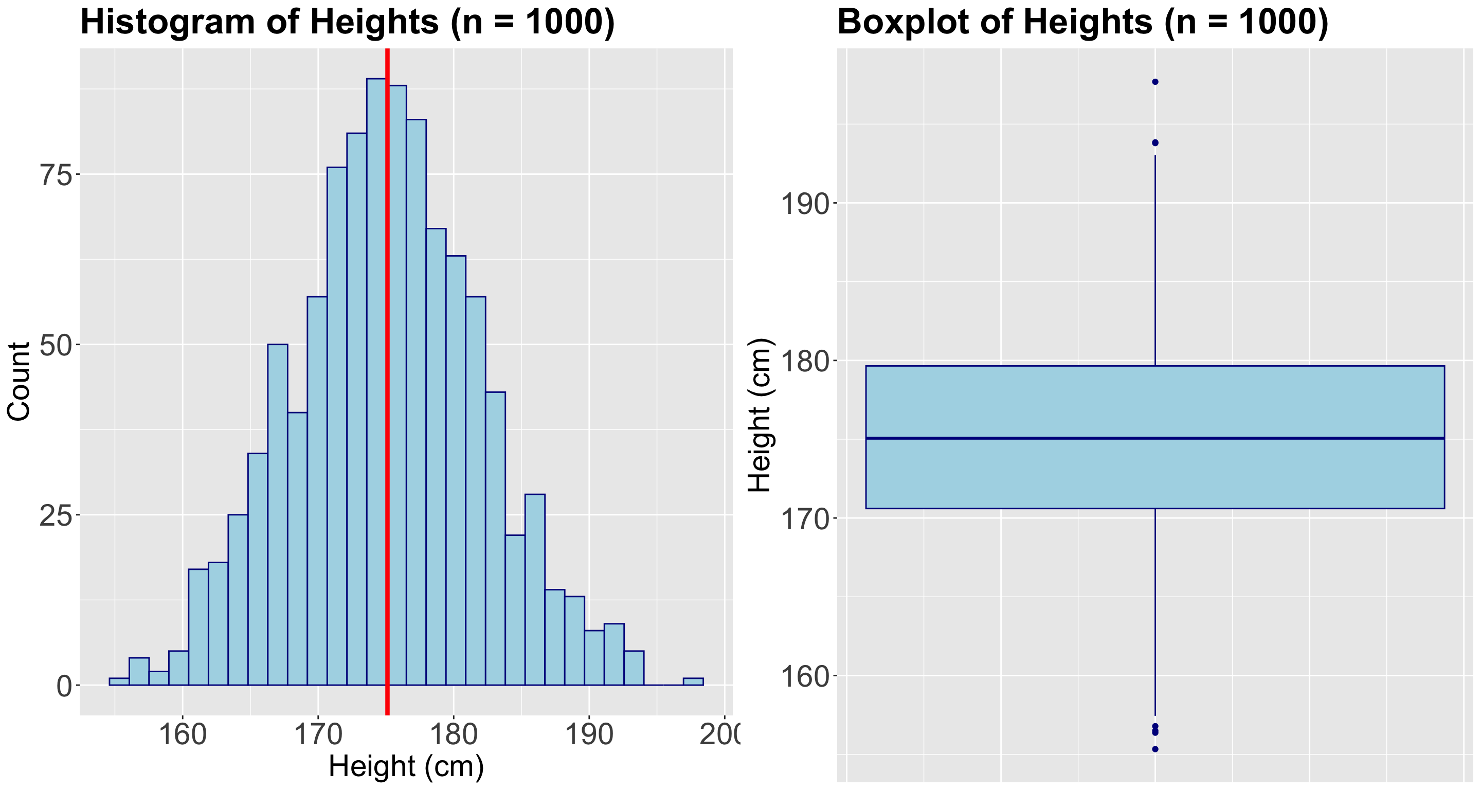
sample_heights <- draw_sample(1000)
sample_mean <- mean(sample_heights)

round(sample_mean,2)

[1] 175.11

In-Class Question (a.k.a. Think-Pair-Share)

• By only using that single sample average, try to answer the following:

1. How much do you know about the distribution of these heights?
2. Is it a symmetric distribution?
3. Is it a heavy-tailed-distribution?
4. What is the variance of this distribution?

Summary of data

• Hence, let us get more information from the sample via summary() and var().

summary(sample_heights)

   Min. 1st Qu.  Median    Mean 3rd Qu.    Max. 
  155.3   170.6   175.1   175.1   179.7   197.7 

paste("variance: ", round(var(sample_heights),2))

[1] "variance:  48.19"

iClicker Question

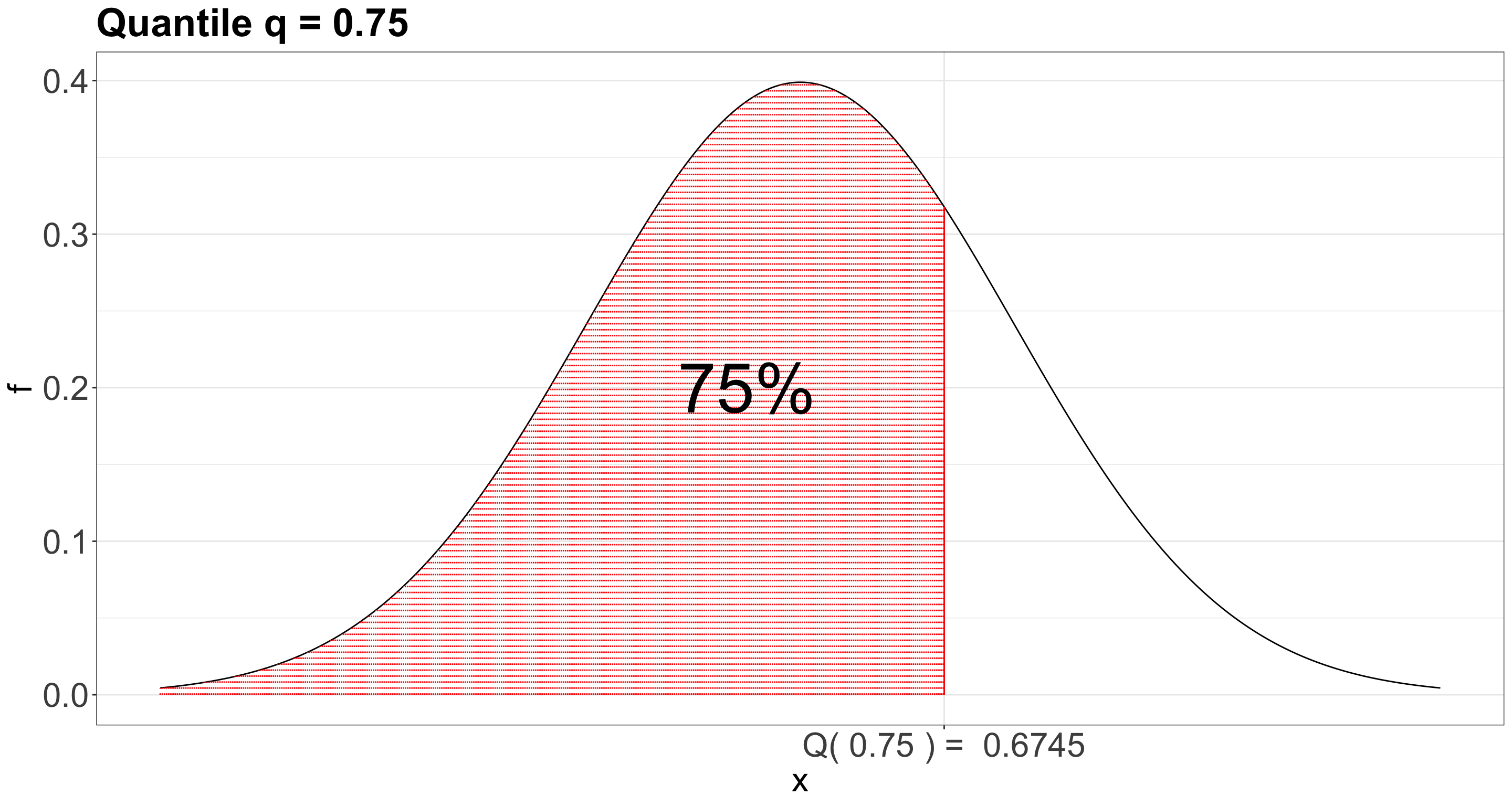
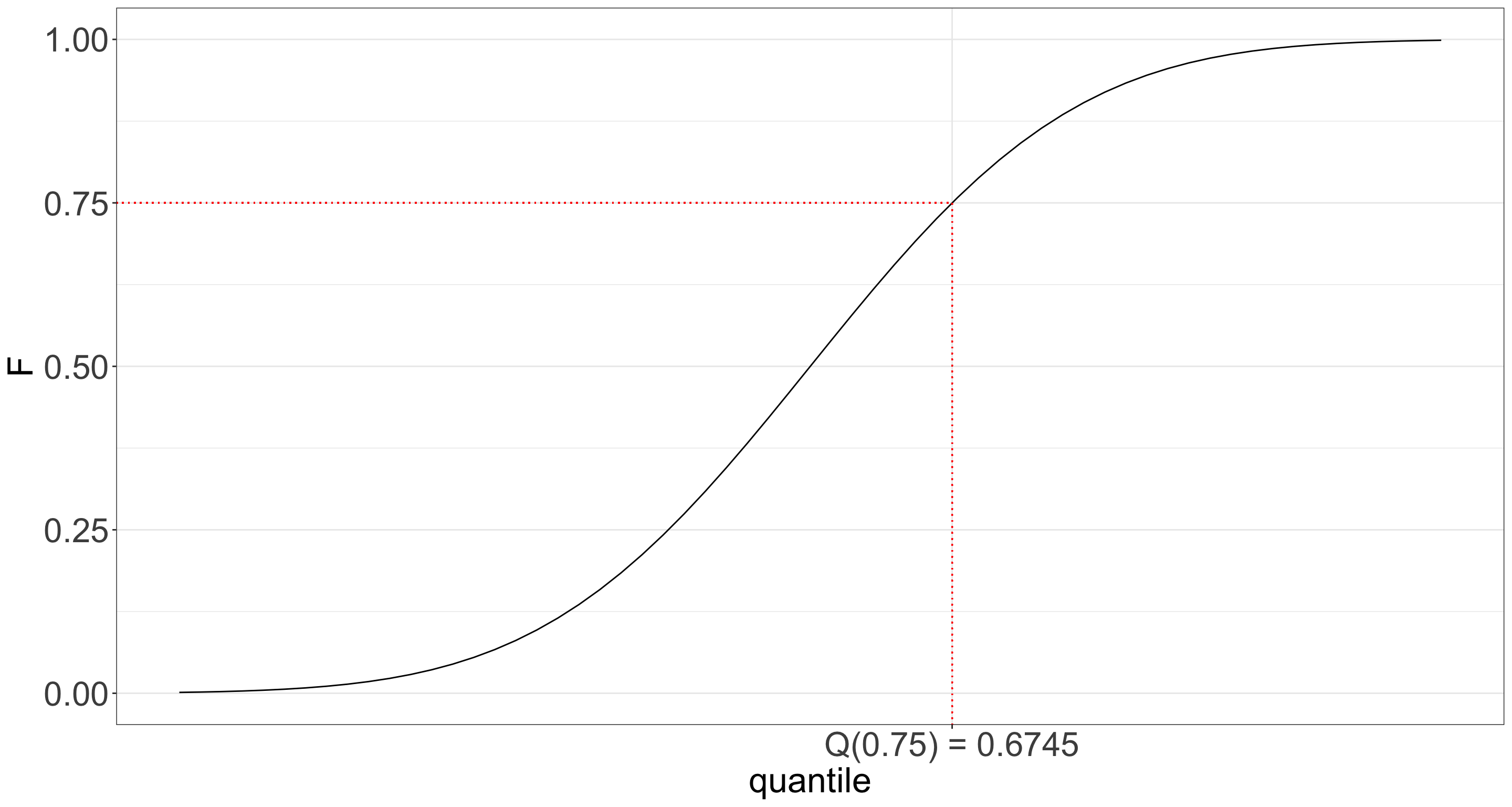
What about now? Do we have a better idea about the distribution?

A. Yes, having different quantiles gives us a better idea about the distribution of heights.

B. Not, at all!

Plot!

1.1. Let us recall what a quantile is!

• Suppose we have a random variable \(X\sim F_X(\cdot)\), i.e., \(X\) has a cumulative distribution function (CDF) \(F_X(\cdot)\).
• Then, the \(\tau\)-quantile (\(0\leq \tau \leq 1\)), is given by \(Q(\tau)\) such that \[\begin{align} F_X[Q(\tau)]= P[X\leq Q(\tau)] = \tau. \end{align}\]

• In plain words, the quantile \(Q(\tau)\) is that observed value of \(X\) for which \(\tau \times 100\%\) of the population’s data is below (or the area under the curve on the left-hand side of a given \(x\)).

As an example …

• We can check the case of the 0.75-quantile in the Standard Normal distribution using its probability density function (PDF).

Moreover…

• We can also show it using the CDF where the cumulative probabilities are on the \(y\)-axis.

1.2. Motivation for Quantile Regression

• In the OLS regression model, we were focused on the conditional mean on the regressors:

\[ \mathbb{E}(Y_i \mid X_{i,j} = x_{i,j}) = \beta_0 + \beta_1 x_{i,1} + \ldots + \beta_k x_{i,k} \; \; \; \; \text{since} \; \; \; \; \mathbb{E}(\varepsilon_i) = 0. \]

• Moreover, we discussed that (from the statistical point of view) regression models follow a stochastic relation.

Plot!

Nonetheless…

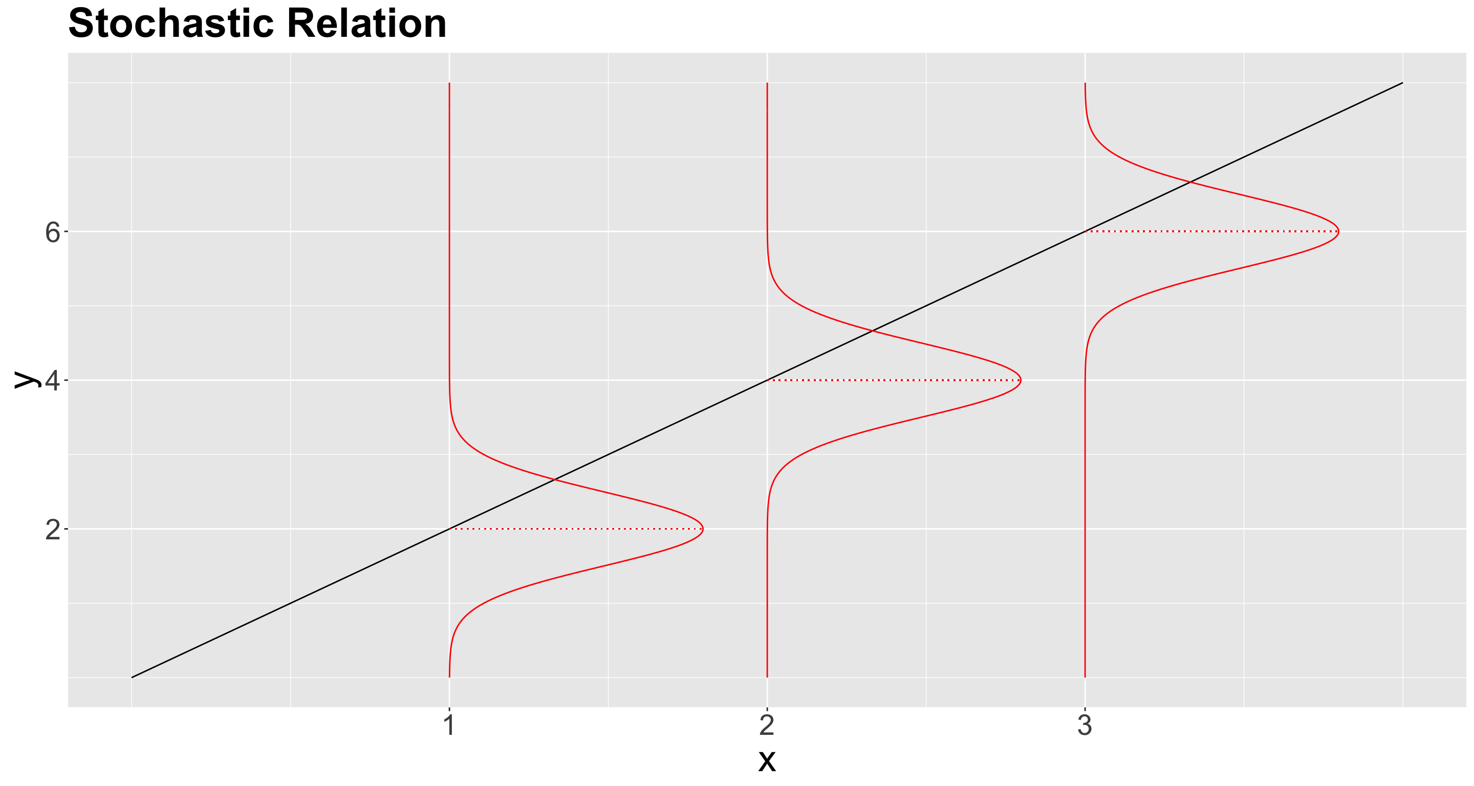
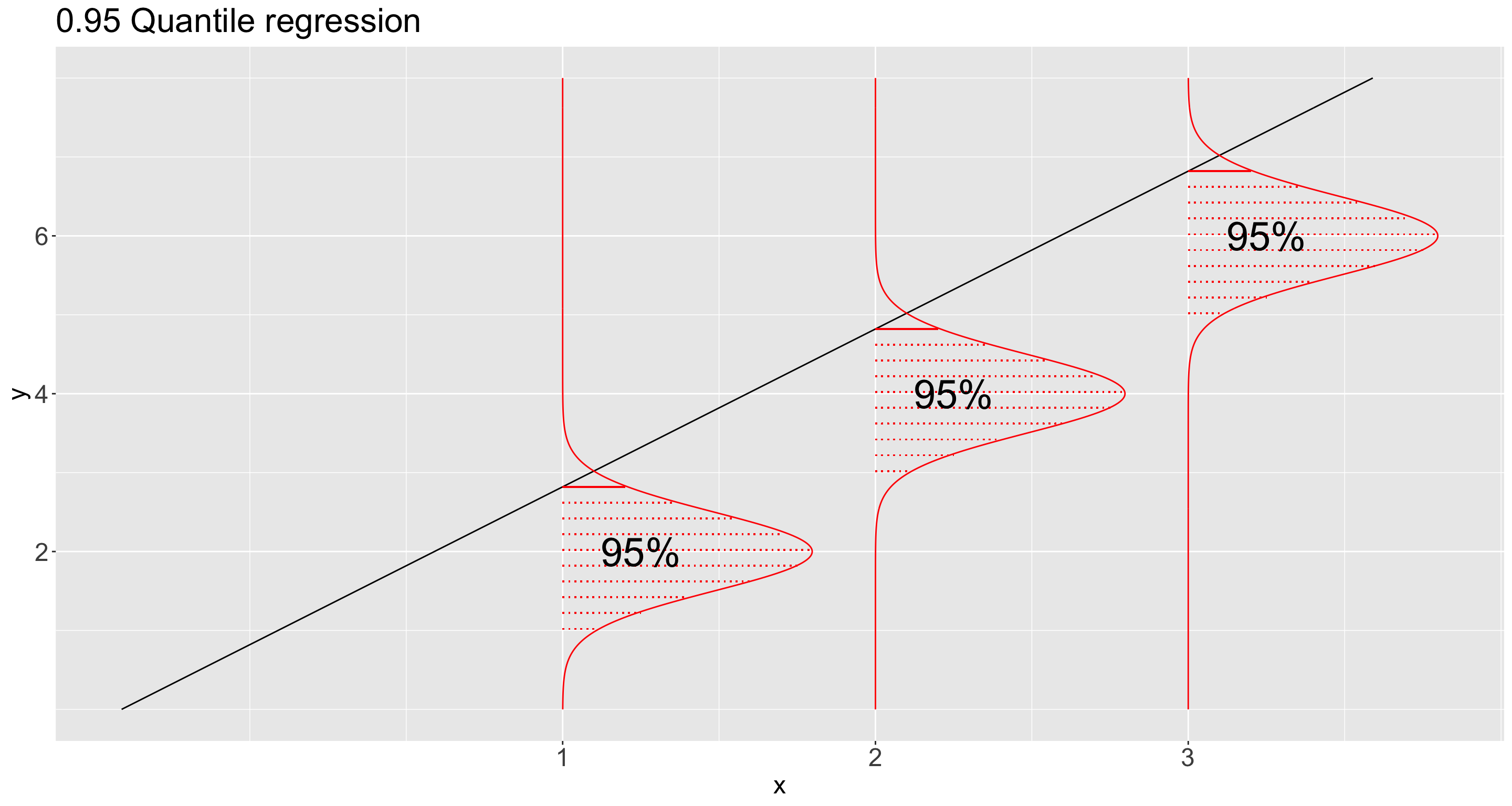
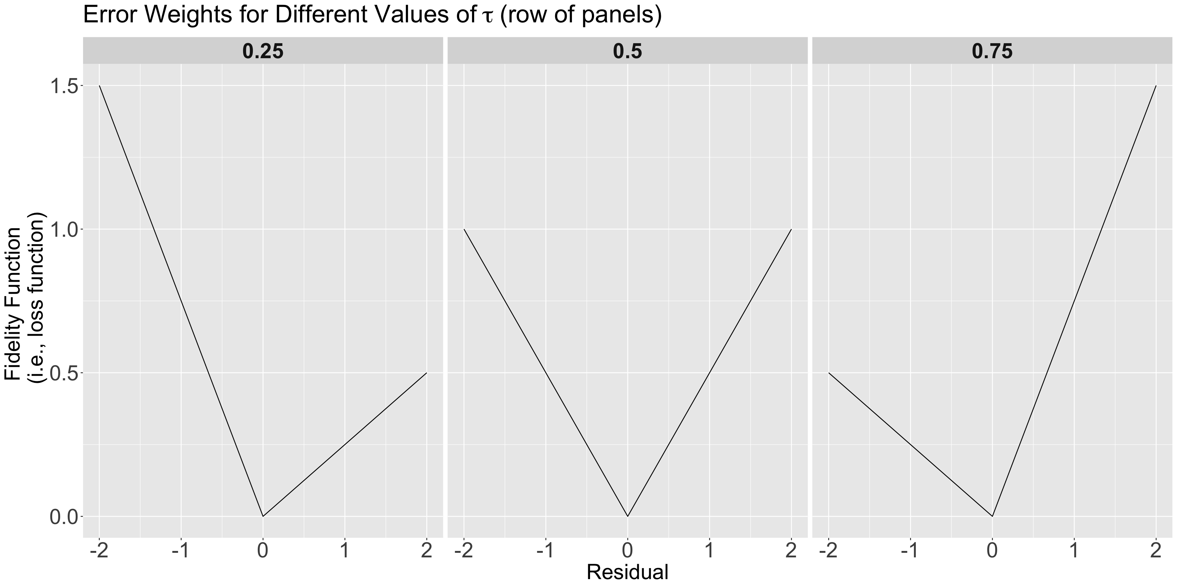
Is it possible to go beyond the conditioned mean?

• Given the stochastic nature of the relation between the response and explanatory variables, we have a whole conditional distribution of the response \(Y_i\), given the \(k\) explanatory variables \(X_{i,j}\) (i.e, regressors).

A conditioned \(0.95\)-quantile!

2. Applications of Quantile Regression

• In many practical cases, we have inferential questions that are related to quantiles and not the mean.
• We might want to see if, at different levels, the response is affected differently by the explanatory variables:

How do driver’s years of experience affect buses’ travel time when considering the 25% fastest travels, 50% fastest travels, and 90% fastest travels?

How does the alcohol price affect the weekly consumption of light drinkers, moderate drinkers, and heavy drinkers at given cut-off values of alcohol consumption?

Furthermore…

• We might also be interested in a probabilistic prediction:

During December in Vancouver, with a 95% chance, what is the maximum snowfall threshold?

Furthermore (Cont’d)

• Note we can translate these inquiries with \(\tau\)-quantiles (\(\tau \in [0, 1]\)) along with the regressor \(X\) and response \(Y\):

How do driver’s years of experience (\(X\)) affect buses’ travel time (Y) when considering the 25% fastest travels (\(\tau = 0.25\)), 50% fastest travels \((\tau = 0.5)\), and 90% fastest travels (\(\tau = 0.9\))?

How does the alcohol price (\(X\)) affect the weekly consumption (\(Y\)) of light drinkers (\(\tau = 0.25\)), moderate drinkers (\(\tau = 0.5\)), and heavy drinkers \((\tau = 0.9)\) in given cut-off values in weekly alcohol consumption?

During December (\(X\)) in Vancouver, with a 95% (\(\tau = 0.95\)) chance, what is the maximum snowfall (\(Y\)) threshold?

2.1. The Teams Dataset

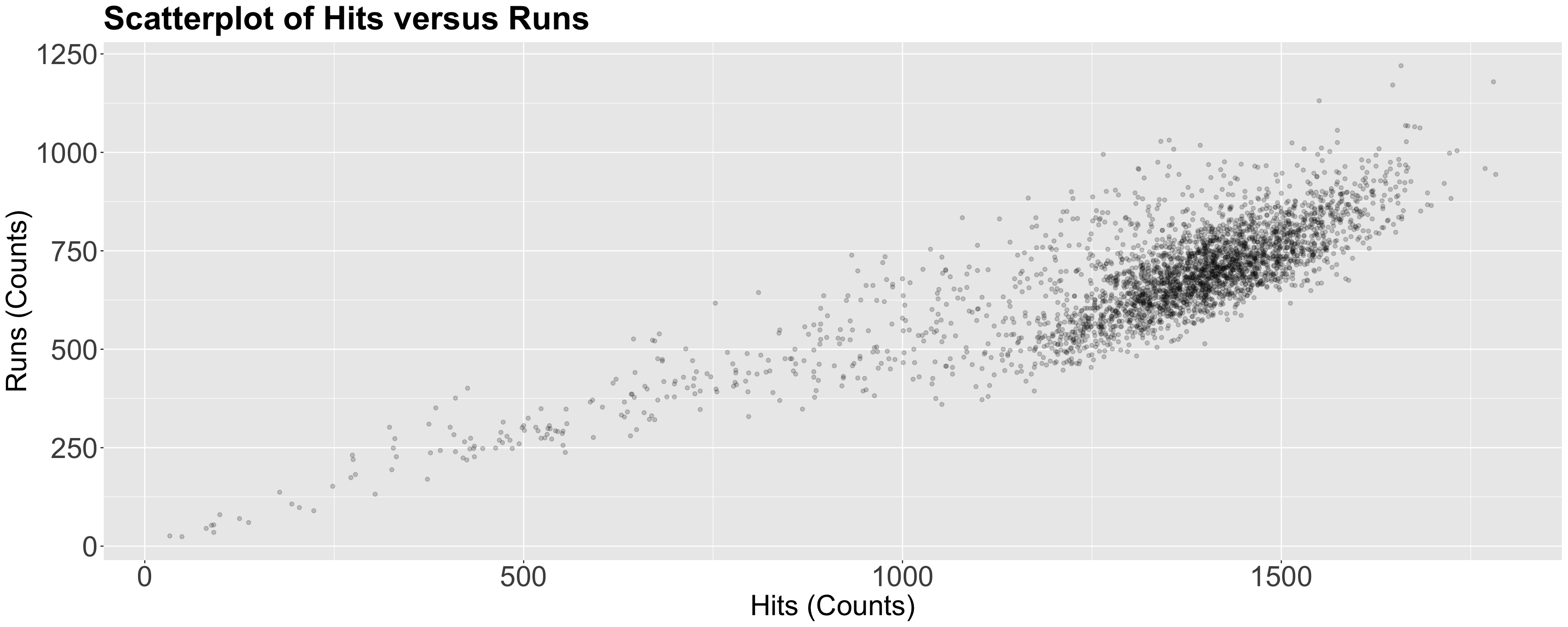
• We will use the Teams dataset from the Lahman package.
• It has \(n = 3075\) observations of 48 variables related to yearly statistics and standings for teams (one row per team) from different American baseball leagues.

Quick data wrangling!

• We will use the following columns:
  • runs: Runs scored, a count-type variable.
  • hits: Hits by batters, a count-type variable.

Main Statistical Inquiries

• You are interested in determining the following using this recorded data:
  1. Previous research has shown you that a large number of runs is associated with a large number of hits. Having said that, for those teams at the upper 75% threshold in runs, is this association significant? If so, by how much?
  2. For any given team that scores 1000 hits in a future tournament, how many runs can this team score with a 50% chance (centred around this future tournament’s median runs)?

2.2. Exploratory Data Analysis

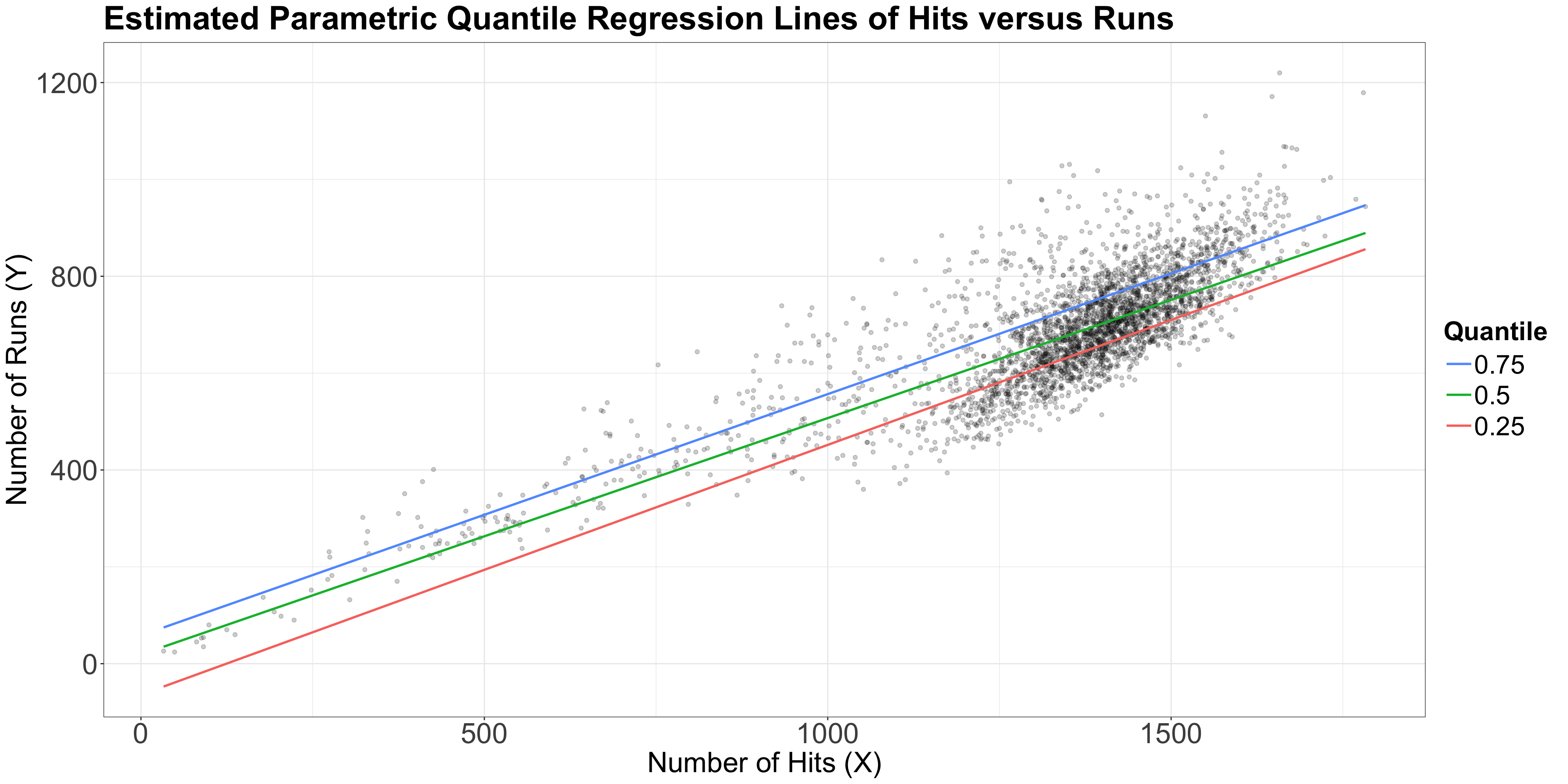
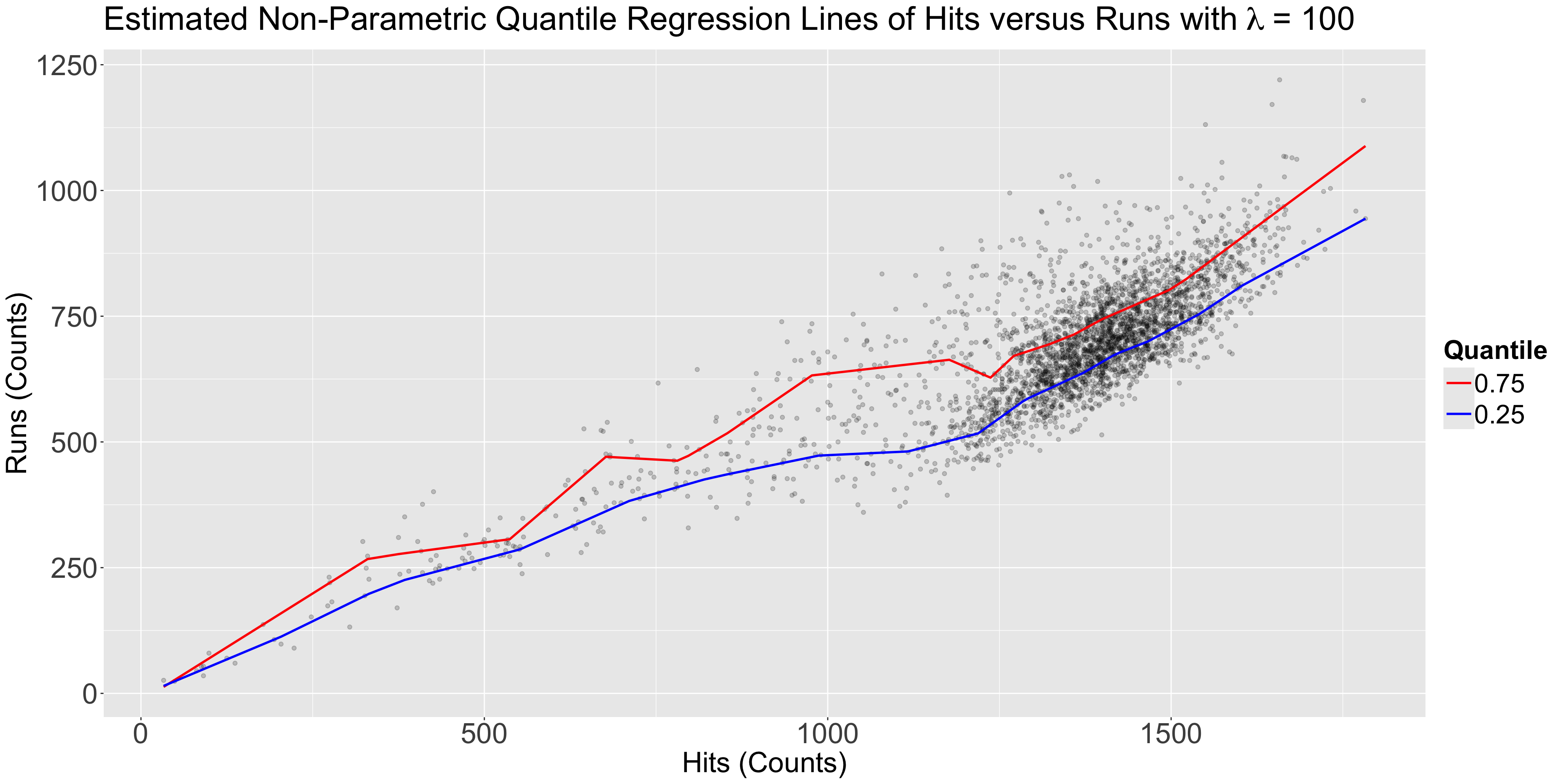
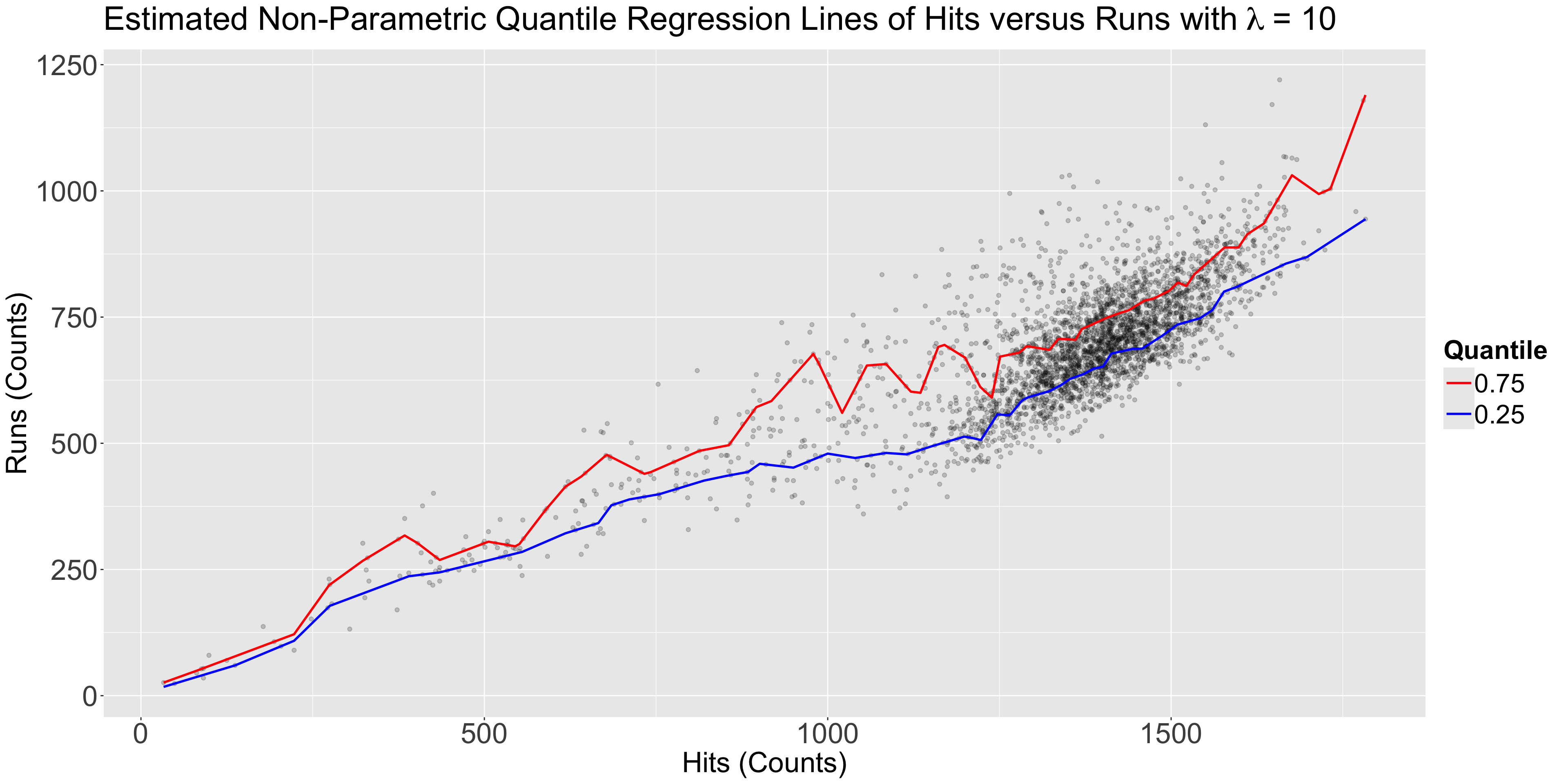
Let us create a scatterplot of hits (our regressor) versus runs (our response), even though these variables are not continuous.

3. Parametric Quantile Regression

• We can address inquiries (1) and (2) via parametric Quantile regression.

• But before digging into this model, it is necessary to recall some fundamentals from OLS.
• In OLS, we use a linear combination on the right-hand side to explain the conditioned mean

\[ \mathbb{E}(Y_i \mid X_{i,j} = x_{i,j}) = \beta_0 + \beta_1 x_{i,1} + \ldots + \beta_k x_{i,k}. \]

Then…

• We find \(\hat{\beta}_0, \hat{\beta}_1, \dots, \hat{\beta}_k\) that minimize the squared error (loss function) in our training set of size \(n\): \[ \sum_{i = 1}^n (y_i - \beta_0 - \beta_1 x_{i,1} - \ldots - \beta_k x_{i,k})^2. \]

3.1. General Modelling Framework

• Suppose we have a random sample (or training data) of size \(n\) with responses \(Y_1, Y_2, \dots, Y_n\) where \(i = 1, 2, \dots, n\).
• Each \(i\)th response is subject to \(k\) regressors \(X_{i, 1}, X_{i, 2}, \dots, X_{i, k}.\)
• Furthermore, we are interested in modelling the response’s \(\tau\)-quantile, where \(\tau \in [0, 1]\), conditioned on these \(k\) regressors in a linear combination with an intercept \(\beta_0(\tau)\) and \(k\) regression coefficients \(\beta_1(\tau), \beta_2(\tau), \dots, \beta_k(\tau)\).

The equation!

\[ Y_i = \underbrace{\beta_0(\tau) + \beta_1(\tau) X_{i,1} + \beta_2(\tau) X_{i,2} + \ldots + \beta_k(\tau) X_{i,k}}_{\text{Systematic Component}} + \underbrace{\varepsilon_i(\tau).}_{\text{Random Component}} \]

• \(\beta_j(\tau)\) (for \(j = 0, 1, 2, \dots, k\)) means that the regression term depends on the quantile \(\tau\), which is the desired quantile.
• For each quantile, we (might if our inquiry dictates so!) have a different regression function on the right-hand side of our modelling equation.
• We still have a distribution-agnostic random component for the \(i\)th observation represented as \(\varepsilon_i(\tau)\), which also depends on the quantile \(\tau\).

Some mathematical rearrangements!

\[\begin{gather*} \varepsilon_i(\tau) = Y_i - \underbrace{\left[ \beta_0(\tau) + \beta_1(\tau) X_{i,1} + \beta_2(\tau) X_{i,2} + \ldots + \beta_k(\tau) X_{i,k} \right]}_{\text{Systematic Component}}. \end{gather*}\]

• Quantile regression must ensure the following global condition: \[ P \left[ \varepsilon_i(\tau) < 0 \mid X_{i, 1}, X_{i, 2}, \dots, X_{i, k} \right] = \tau. \]

In a more practical setting…

• Suppose you use the teams dataset to fit a Quantile regression of runs (\(Y\)) versus hits (\(X_1\)) on the response’s quantile \(\tau = 0.75\).
• Then, your regression equation for the \(i\)th observation becomes: \[ Y_i = \underbrace{\beta_0(\tau = 0.75) + \beta_1(\tau = 0.75) X_{i,1}}_{\text{Systematic Component}} + \underbrace{\varepsilon_i(\tau = 0.75).}_{\text{Random Component}} \]

• This yields \[\begin{gather*} \varepsilon_i(\tau = 0.75) = Y_i - \underbrace{\left[ \beta_0(\tau = 0.75) + \beta_1(\tau = 0.75) X_{i,1} \right]}_{\text{Systematic Component}} \qquad \text{with} \\ P \left[ \varepsilon_i(\tau = 0.75) < 0 \mid X_{i, 1} \right] = \tau = 0.75. \end{gather*}\]

The estimated Quantile Regression Line with \(\hat{\beta_0}(\tau = 0.75)\) and \(\hat{\beta_1}(\tau = 0.75)\)

Summarizing…

• A parametric Quantile regression will condition the \(\tau\)-quantile (\(\tau \in [0, 1]\)) to \(k\) regressors in a linear combination with an intercept \(\beta_0(\tau)\) and \(k\) regression coefficients: \[ Q_i( \tau \mid X_{i,j} = x_{i,j}) = \beta_0(\tau) + \beta_1(\tau) x_{i,1} + \ldots + \beta_k(\tau) x_{i,k}. \]

• This is analogous to the conditional expected value that OLS aims to model such as: \[ \mathbb{E}(Y_i \mid X_{i,j} = x_{i,j}) = \beta_0 + \beta_1 x_{i,1} + \ldots + \beta_k x_{i,k}. \]

Heads-up!

• Parametric Quantile regression will aim to find \(\hat{\beta}_0(\tau), \hat{\beta}_1(\tau), \dots, \hat{\beta}_k(\tau)\) that minimize the following error function (loss function): \[\begin{equation*} \sum_{i} e_i[\tau - I(e_i < 0)] = \sum_{i: e_i \geq 0} \tau|e_i|+\sum_{i: e_i < 0}(1-\tau)|e_i|. \end{equation*}\]

• Unlike OLS, where there is a single model fitting, any Quantile regression approach (either parametric or non-parametric) would require fitting as many models as quantiles we are interested in!

Some notes!

• In the previous loss function we have the indicator variable: \[\begin{equation*} I(e_i < 0) = \begin{cases} 1 \; \; \; \; \mbox{if $e_i$ < 0},\\ 0 \; \; \; \; \mbox{otherwise;} \end{cases} \end{equation*}\]
• The residual is defined as: \[\begin{gather*} e_i = y_i - \overbrace{\big[\hat{\beta_0}(\tau) + \hat{\beta_1}(\tau) x_{i,1} + \ldots + \hat{\beta_k}(\tau) x_{i,k}\big]}^{\hat{y_i}} \\ e_i = y_i - \hat{y_i} \end{gather*}\]
• This error function is called fidelity (also known as check function or pinball loss function).

Now…

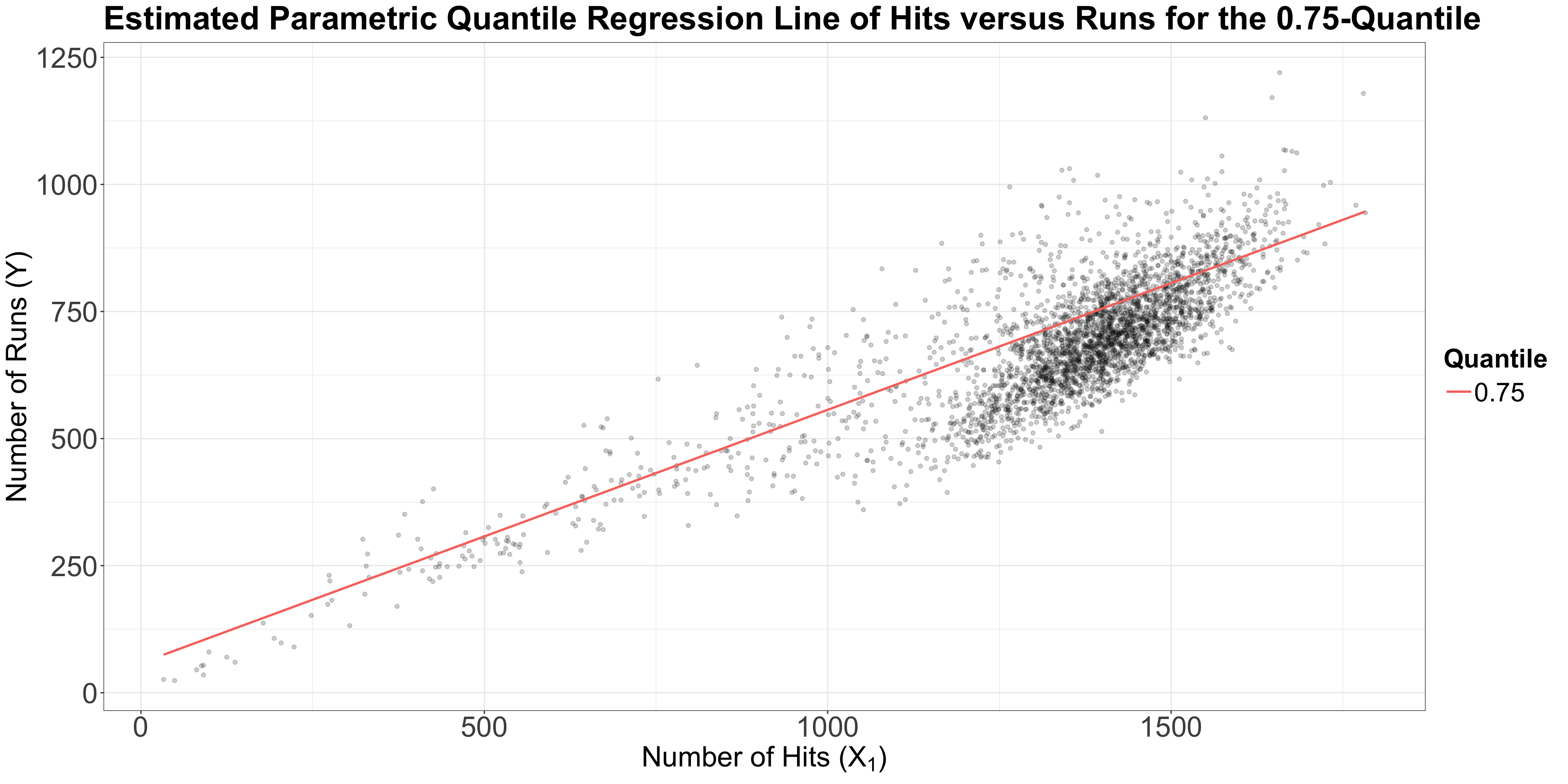
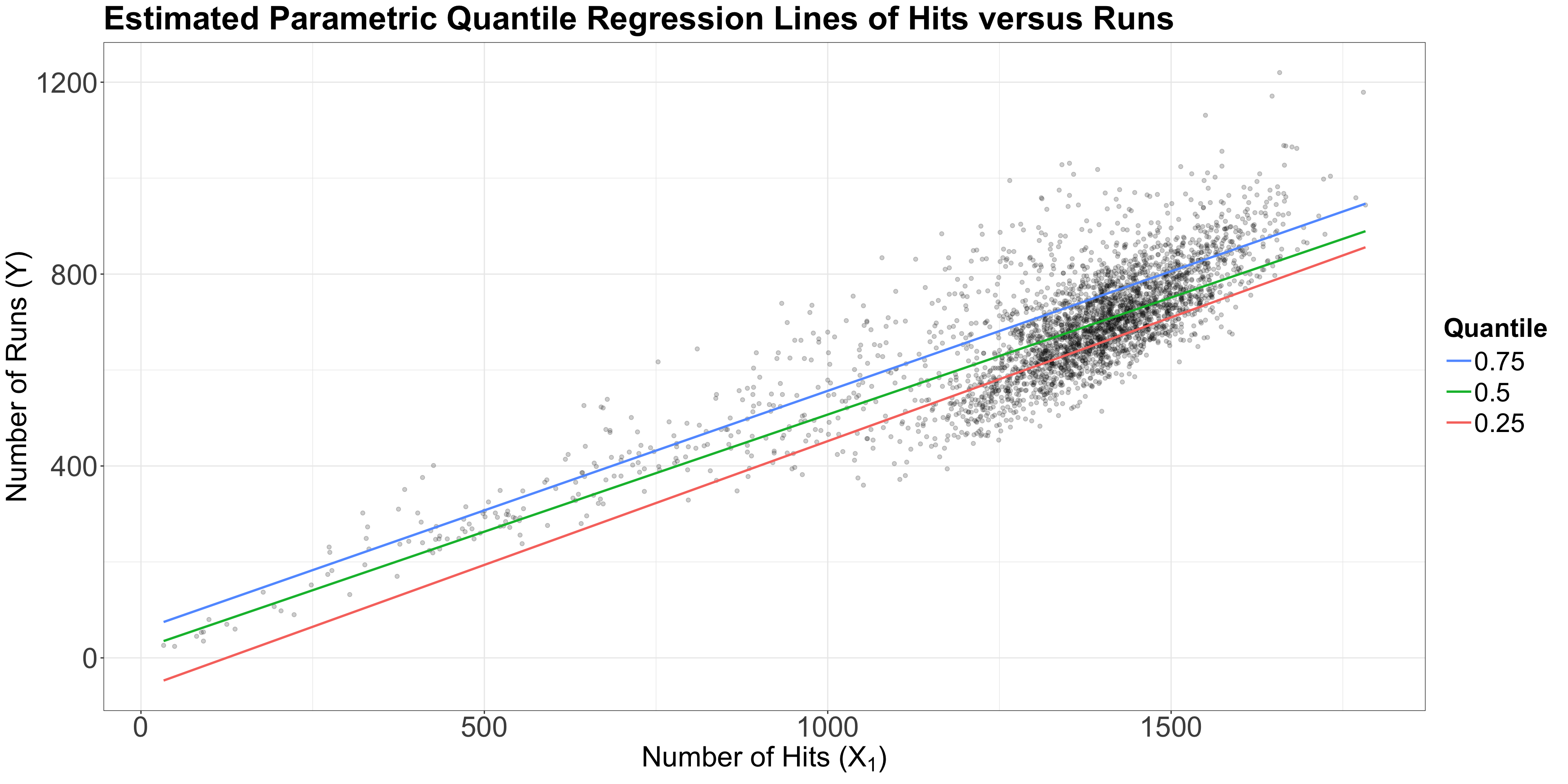
• To understand how the fidelity function works, using the teams dataset, let us plot the three estimated parametric Quantile regression lines for quantiles \(\tau = 0.25, 0.5, 0.75\).
• Our response \(Y\) is runs, whereas our regressor \(X_1\) is hits.

Plot!

Heads-up!

• A fundamental characteristic of a \(\tau\)-Quantile regression (either parametric or non-parametric) is that we will practically have the \(\tau \times 100\%\) of our observed responses below our estimated regression line via \(\hat{\beta}_0(\tau), \hat{\beta}_1(\tau), \dots, \beta_k(\tau)\).

How does the fidelity function behave?

• Let us assume we have the same set of regressor values \(x_{i,1}, \dots, x_{i,k}\) in the following panels for \(\tau = 0.25, 0.5, 0.75\).
• Moreover, we will have the corresponding set of estimates \(\hat{\beta}_0(\tau), \hat{\beta}_1(\tau), \dots, \hat{\beta}_k(\tau)\) by \(\tau = 0.25, 0.5, 0.75\).
• We have the values of the corresponding fidelity function on the \(y\)-axis, whereas we have the corresponding values on the \(x\)-axis for the residual \[\begin{gather*} e_i = y_i - \overbrace{\big[\hat{\beta_0}(\tau) + \hat{\beta_1}(\tau) x_{i,1} + \ldots + \hat{\beta_k}(\tau) x_{i,k}\big]}^{\hat{y_i}} \\ e_i = y_i - \hat{y_i}. \end{gather*}\]

Plots!

From left to right!

\(\tau = 0.25\)

• Recall the residual is \(\quad e_i = y_i - \overbrace{\big[\hat{\beta_0}(\tau) + \hat{\beta_1}(\tau) x_{i,1} + \ldots + \hat{\beta_k}(\tau) x_{i,k}\big]}^{\hat{y_i}}.\)

Note that for low values of \(\tau\), we consider overpredicting \[e_i = y_i - \hat{y_i} < 0\] WORSE than underpredicting \[e_i = y_i - \hat{y_i} > 0.\]

From left to right! (Cont’d)

\(\tau = 0.5\)

• For \(\tau = 0.5\), we care equally about underpredicting and overpredicting.
• This corresponds to the median value.

From left to right! (Cont’d)

\(\tau = 0.75\)

• Recall the residual is \(\quad e_i = y_i - \overbrace{\big[\hat{\beta_0}(\tau) + \hat{\beta_1}(\tau) x_{i,1} + \ldots + \hat{\beta_k}(\tau) x_{i,k}\big]}^{\hat{y_i}}.\)

Note that for high values of \(\tau\), we consider underpredicting \[e_i = y_i - \hat{y_i} > 0\] WORSE than overpredicting \[e_i = y_i - \hat{y_i} < 0.\]

Plot!

3.2. Estimation

• If our linear systematic component has \(k\) regression parameters (intercept AND coefficients), then our estimated Quantile regression function will interpolate \(k + 1\) points.

• For example, if we are fitting a line \(Q_i( \tau | X = x_i) = \beta_0(\tau) + \beta_1(\tau) x_i\), we are estimating two parameters (\(\hat{\beta_0}\) and \(\hat{\beta_1}\)). So, our fitted line is a line that passes through two points.
• As we already mentioned, when we use the \(\tau\)-quantile with a training set of size \(n\), approximately \(n \times \tau\) points will be under the curve and \(n \times (1 - \tau)\) will be above the curve.

For instance…

• If we have \(n = 100\) points to fit the \(0.7\)-quantile, then:

  • The number of points above the line will be approximately 30.
  • The number of points below the line will be approximately 70.

• The “approximately” comes because we will have \(k + 1\) points ON the estimated regression function.
• Let us consider the teams dataset again. In this example, we will estimate the quantiles of runs as a linear function of hits. We can obtain these estimated \(0.25\), \(0.5\), and \(0.75\)-quantile regression lines via geom_quantile().

The code!

estimated_quantile_regression_lines <- ggplot(teams, aes(hits, runs)) +
  geom_point(alpha = 0.2, colour = "black") +
  geom_quantile(
    quantiles = c(0.25, 0.5, 0.75), aes(colour = as.factor(after_stat(quantile))),
    formula = y ~ x, linewidth = 1
  ) +
  theme_bw() +
  labs(
    x = "Number of Hits (X)",
    y = "Number of Runs (Y)"
  ) +
  theme(
    plot.title = element_text(size = 30, face = "bold"),
    axis.text = element_text(size = 26),
    axis.title = element_text(size = 26),
    legend.text = element_text(size = 24, margin = margin(r = 1, unit = "cm")),
    legend.title = element_text(size = 24, face = "bold"),
    legend.key.size = unit(1, "cm")
  ) +
  guides(colour = guide_legend(title = "Quantile", reverse = TRUE)) +
  ggtitle("Estimated Parametric Quantile Regression Lines of Hits versus Runs")

Plot!

Fit the model in R!

• Via the {quantreg} package, we will use the rq() function to fit the parametric Quantile regression at \(\tau = 0.25, 0.5, 0.75\).
• It has a formula argument as the previous fitting functions along with data.
• This function also allows us to fit as many Quantile regressions as we want via tau.

A quick note on the standard errors and \(p\)-values!

• There is more than one way to obtain the standard errors and \(p\)-values of the regression estimates.
• For the purpose of this course, we will use the pairwise bootstrapping method via the arguments se = "boot" and bsmethod = "xy".
• Specifically, for this example, we will use R = 1000 replicates in function summary().

Modelling Output

3.3. Inference

• We can determine whether a regressor is statistically associated with the \(\tau\)-quantile in our response through hypothesis testing for \(\beta_j(\tau)\).
• We will need the estimated regression coefficient \(\hat{\beta_j}(\tau)\) and its bootstrapped standard error, \(\mbox{se}\left[\hat{\beta_j}(\tau) \right]\).
• You can test the below hypotheses via the test statistic \(t_j = \frac{\hat{\beta_j}(\tau)}{\mbox{se}\left[\hat{\beta_j} (\tau) \right]}\): \[\begin{align*} H_0: \beta_j(\tau) &= 0 \\ H_a: \beta_j(\tau) &\neq 0. \end{align*}\]

Reminder!

• Let us recall our inquiry (1):

Previous research has shown you that a large number of runs is associated with a large number of hits. Having said that, for those teams at the upper 75% threshold in runs, is this association significant? If so, by how much?

• Note that this inferential question corresponds to the estimated \(0.75\)-Quantile regression.

Solving the inquiry!

Our sample gives us evidence to reject \(H_0\) with a \(p\text{-value} < .001\). So hits is statistically associated to the \(0.75\)-quantile of runs.

3.4. Coefficient Intepretation

• We can quantify the statistical association of hits and the \(0.75\)-quantile of runs via the corresponding \(\hat{\beta_1}(0.75)\).

• The interpretation is: “for each one hit increase, the \(0.75\)-quantile of runs will increase by 0.5.”

3.5. Predictions

• Now, let us check our inquiry (2):

For any given team that scores 1000 hits in a future tournament, how many runs can this team score with a 50% chance (centred around this future tournament’s median runs)?

Then…

• We can obtain this prediction via our \(0.25\) and \(0.75\)-Quantile regressions with predict().

Finally…

• Our predictive inquiry can be answered as: “for any given team that scores 1000 hits in a future tournament, it is estimated to have a 50% (\(0.75 - 0.25 \times 100\%\)) chance to have between 452 and 556 runs.”
• This is a probabilistic prediction!
• Note we could also say that this team:
  • has a 25% (\(1 - 0.75 \times 100\%\)) chance of achieving over 556 runs,
  • has a 25% (\(0.25 \times 100\%\)) chance of getting less than 452 runs,
  • and would typically get 507 runs (median).

4. Non-Parametric Quantile Regression

• The predictive inquiry (2) can also be dealt with via non-parametric Quantile regression.
• This class of Quantile regression implicates no distributional assumptions and no model function specification. It is a method based on splines.
• The core idea is to allow the model to capture the local behaviour of the data (i.e., capturing its local structure).

4.1. General Modelling Framework

• The struggle is choosing how local our model should be. In other words, what is the neighbourhood of a point \(x\)?

• A parameter will control this. We will call it lambda, a penalization parameter:
  • A small neighbourhood (i.e., a small lambda) will provide a better approximation, but with too much variability – we might be prone to overfitting.
  • A too-large neighbourhood (i.e., a big lambda) will lose local information favouring smoothness – we might be prone to underfitting.

4.2. Estimation

• In R, non-parametric Quantile regression is performed using the function rqss() from library quantreg.
• It also works somewhat similarly to what we are used to with the lm() and glm() functions.
• However, in rqss() each regressor must be introduced in the formula using the qss() function (as additive non-parametric terms). For example, qss(x, lambda = 10).

Syntax

• The syntax would be:

rqss(y ~ qss(x, lambda = 10), tau = 0.5, data = my_data)

• We use rqss() to run a non-parametric Quantile regression with runs as the response and hits as the regressor.
• We use a tau = 0.25 and tau = 0.75.
• Note rqss() does not allow multiple values for tau.
• Therefore, we fit a model per tau value. Here, we try a lambda = 100.

Non-parametric Quantile Regression for \(\tau = 0.25\)

Non-parametric Quantile Regression for \(\tau = 0.75\)

Then…

• We plot the two model functions on the data plot. This is basically our prediction band (which can also apply to our parametric models!).

Plot!

What if we use lambda = 10?

Next model!

Plot!

A quick check!

• As a sanity check, let us calculate the proportion of points below these estimated regression functions with \(\lambda = 10\).

4.3. Prediction

• Suppose that we go ahead with the non-parametric models with \(\lambda = 10\), then we obtain the corresponding probabilistic interval:

Thus…

• Our predictive inquiry can be answered as:

For any given team that scores 1000 hits in a future tournament, it is estimated to have a 50% \((0.75 - 0.25 \times 100\%)\) chance to have between 491 and 625 runs.

5. Wrapping Up

• We can extend the regression paradigm beyond the conditioned response mean.
• We could assess association (or causation under a proper experimental framework!) via different response statistics such as quantiles to a set of regressors.
• Quantile regression can be non-parametric (more suitable for predictions) or parametric (to allow for coefficient interpretation).