Lecture 8
Missing Data
1.2. Missing At Random (MAR)
- In this type, missingness depends on the observed data we have.
- Therefore, we could use some imputation techniques for this missingness, such as multiple imputation (to be covered later on today), based on the rest of our available data (a hot deck imputation technique).

iClicker Question
Are these higher standard errors related to the MCAR nature of the deleted rows?
A. Yes.
B. No.
Descriptive statistics!
- We will try getting the mean
dep_delaypercarrier,but we have missing data indep_delay, which will return a summary withNAs.

How to handle NA’s?
- Assuming data is MCAR, if we want to make a listwise deletion to get the means by
carrier, we just usena.rm = TRUEinmean().

Nonetheless…
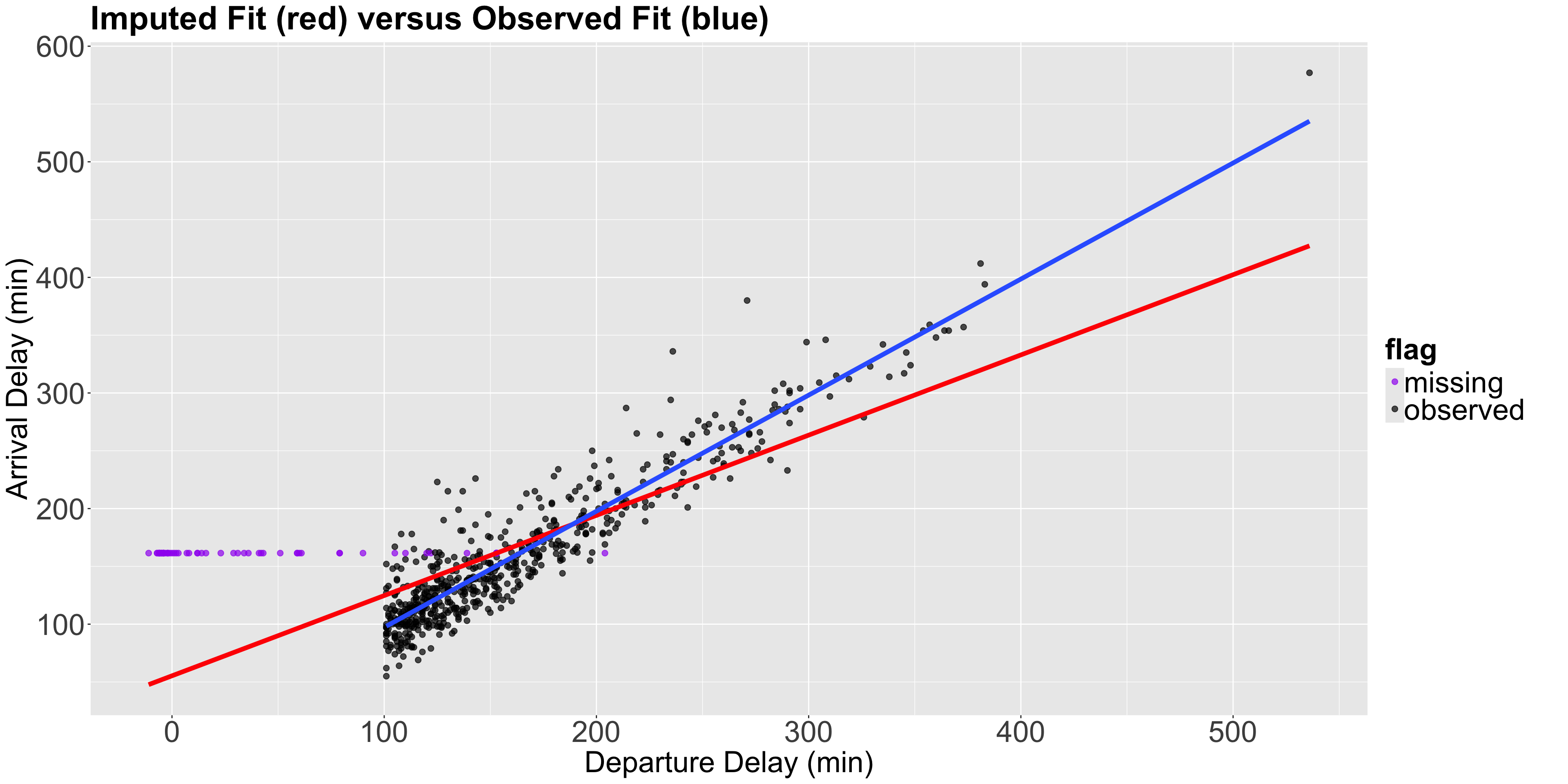
- We have to be careful. If the missing data in
flightsis not MCAR, we can introduce serious bias in our estimates (means in this case) for some given statistical approach. - But, why a bias?
Another Example
- Suppose that people with low income have a higher chance of omitting their income (as a numeric variable) in a given survey used for regression analysis.
- Then, if we just drop those rows, we are skewing our analysis towards people with higher income without knowing. So, there will be a bias in our results in our regression estimates.

iClicker Question
- Let us retake the previous survey example regarding low-income respondents. Suppose this survey collects additional information, such as the respondent’s specific neighbourhood, which is a complete column.
- Then, you could match this extra information with some other neighbourhood databases identifying low, middle, and high-income areas.
- What class of missing data are these missing incomes in the survey?
A. MCAR.
B. MAR.
C. MNAR.
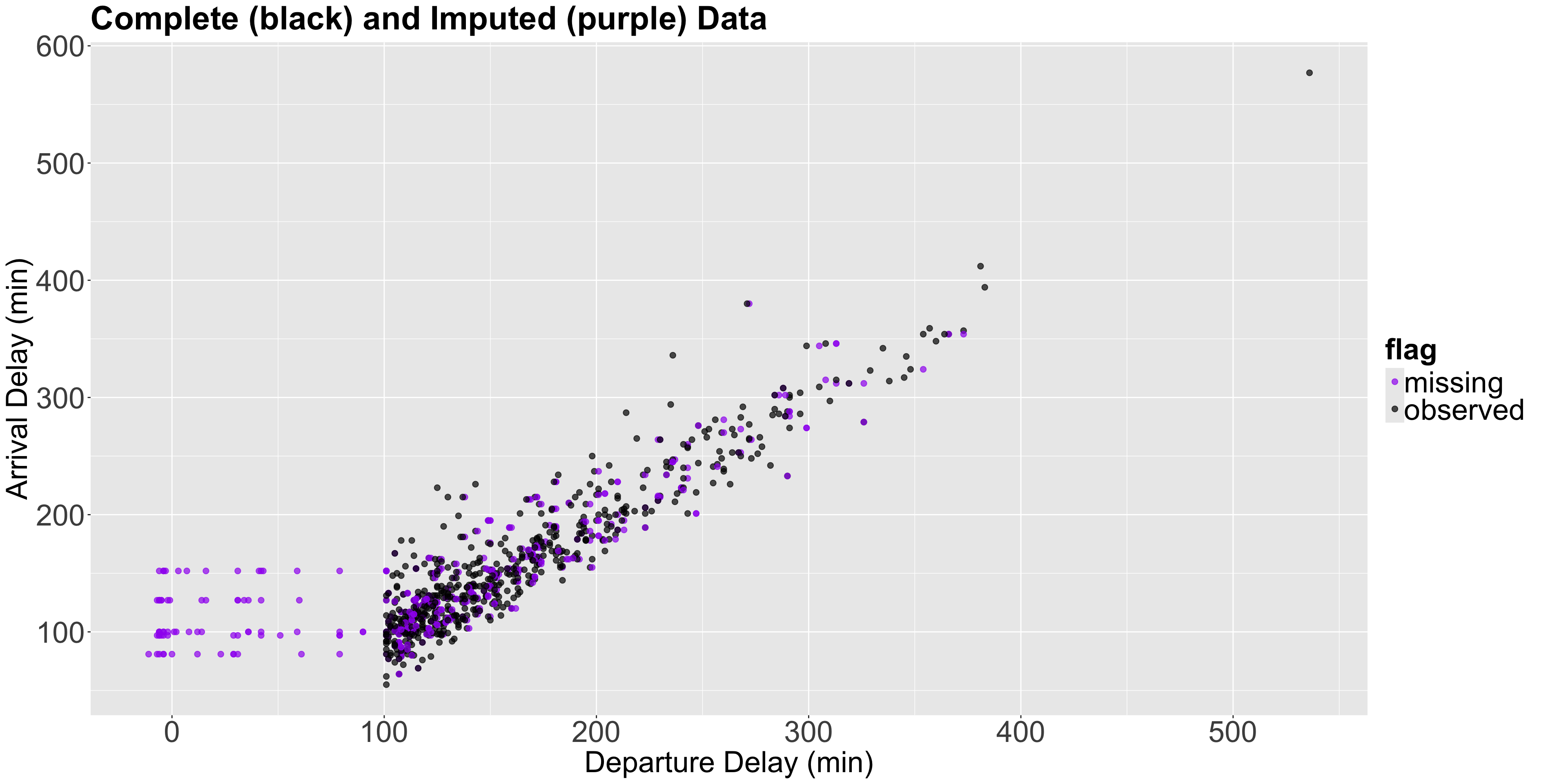
Plot!
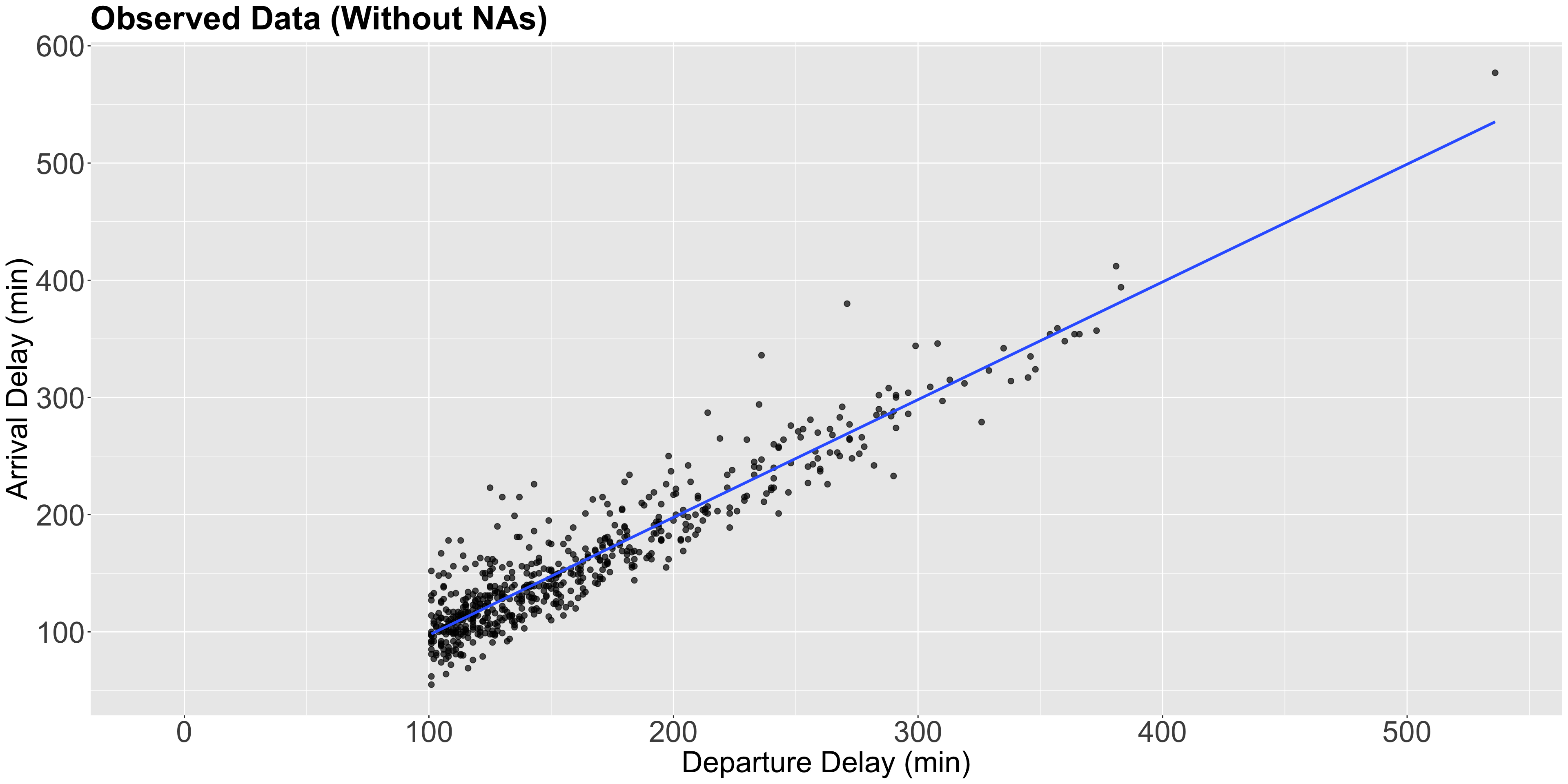
Plot!
Plot!
2.4. Last Observation Carried Over
- Another method that we might see out there is imputing data by repeating the previous observation.
- This is more frequent when dealing with temporal data, and will be out of the scope of this course.

Workflow
- We would use our pooled model, fitted with our response of interest subject to our regressor set, to answer our inferential or predictive inquiries. The below diagram provides a clearer perspective
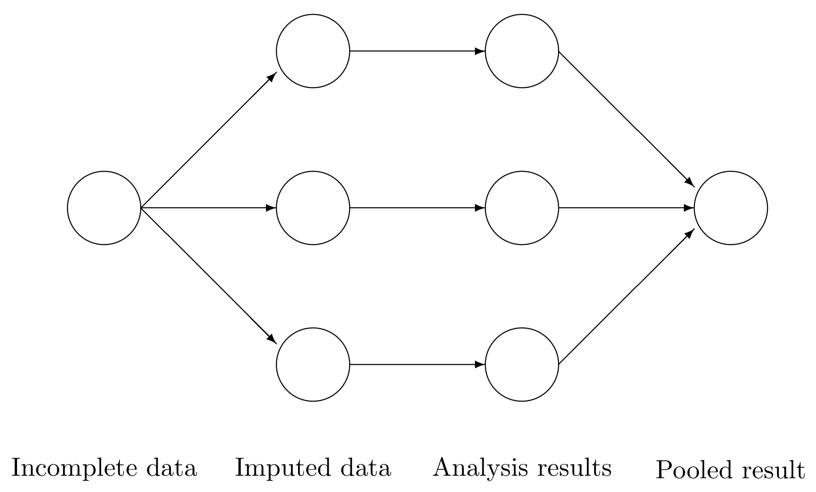
Source: van Buuren (2012).
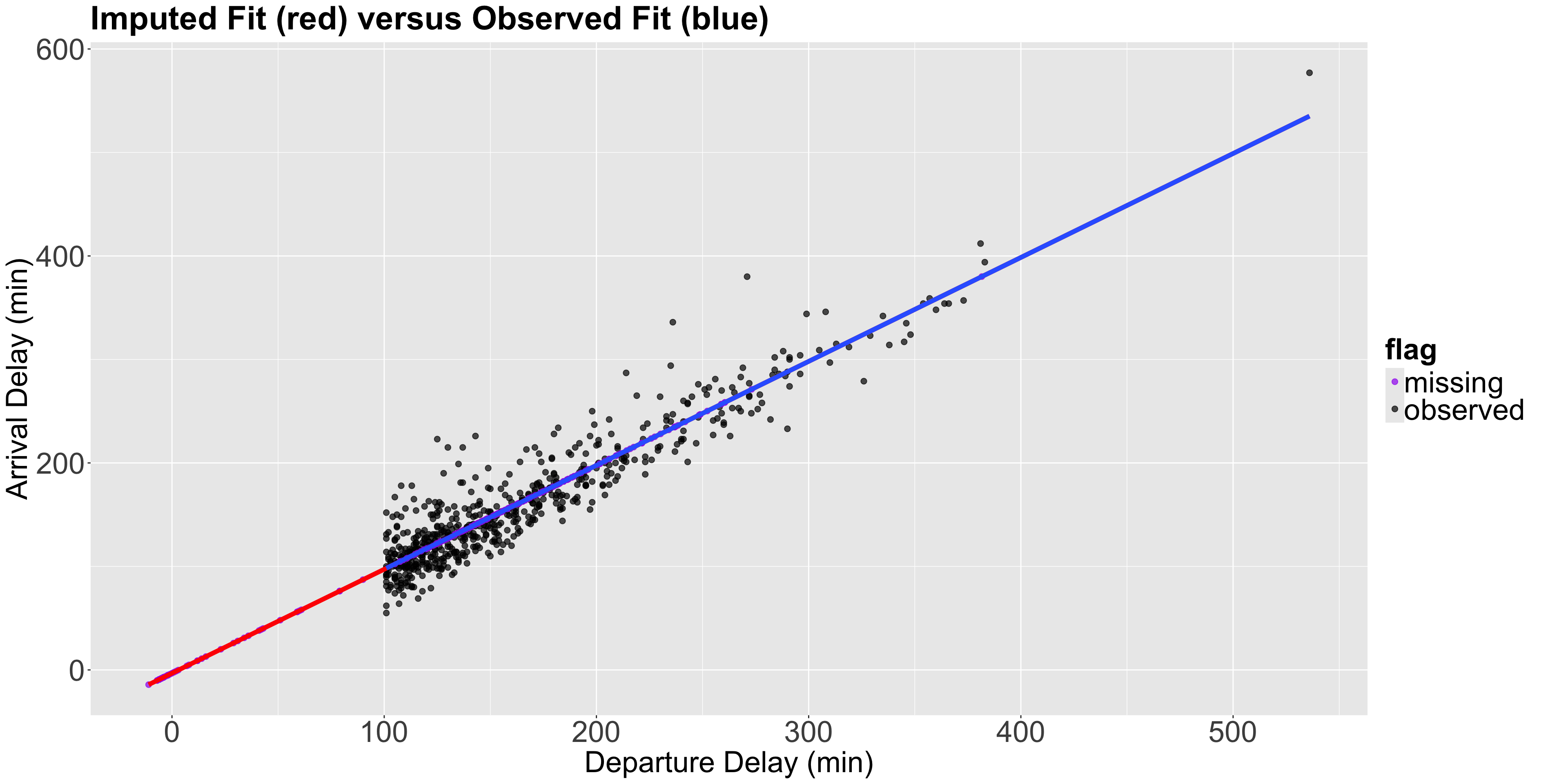
Plot!
3. Wrapping Up
Data imputation involves some wrangling effort and proper missingness visualizations.
We have to be careful when defining our class of data missingness since this will determine the type of data imputation we need to make (or maybe data deletion!).
In general, multiple imputation will work OK for MAR and MNAR data.
We only saw continuous imputation in this example. Nonetheless, the
mice()approach can be extended to other data types such as binary or categorical. In those cases, we have to switch to generalized linear models (GLMs), even with a Bayesian approach.
![]()