Predicting Bank Marketing Success on Term Deposit Subscription

Summary

In this analysis, we attempt to build a predictive model aimed at determining whether a client will subscribe to a term deposit, utilizing the data associated with direct marketing campaigns, specifically phone calls, in a Portuguese banking institution.

After exploring on several models (logistic regression, KNN, decision tree, naive Bayers), we have selected the logistic regression model as our primary predictive tool. The final model performs fairly well when tested on an unseen dataset, achieving the highest AUC (Area Under the Curve) of 0.899. This exceptional AUC score underscores the model’s capacity to effectively differentiate between positive and negative outcomes. Notably, certain factors such as last contact duration, last contact month of the year and the clients’ types of jobs play a significant role in influencing the classification decision [Dwork et al., 2015].

Introduction

In the banking sector, the evolution of specialized bank marketing has been driven by the expansion and intensification of the financial sector, introducing competition and transparency. Recognizing the need for professional and efficient marketing strategies to engage an increasingly informed and critical customer base, banks grapple with conveying the complexity and abstract nature of financial services. Precision in reaching specific locations, demographics, and societies has proven challenging. The advent of machine learning has revolutionized this landscape, utilizing data and analytics to inform banks about customers more likely to subscribe to financial products[Moro et al., 2014]. In this machine learning-driven bank marketing project, we explore how a particular Portuguese bank can leverage predictive analytics to strategically prioritize customers for subscribing to a bank term deposit, showcasing the transformative potential of machine learning in refining marketing strategies and optimizing customer targeting for financial institutions.

Data

Our analysis centers on direct marketing campaigns conducted by a prominent Portuguese banking institution[Moro et al., 2012], specifically phone call campaigns designed to predict clients’ likelihood of subscribing to a bank term deposit. The comprehensive dataset provides a detailed view of these marketing initiatives, offering valuable insights into factors influencing client subscription decisions. The dataset, named ‘bank-full.csv,’ encompasses all examples and 17 inputs, ordered by date. The primary focus of our analysis is classification, predicting whether a client will subscribe (‘yes’) or not (‘no’) to a term deposit, providing crucial insights into client behavior in response to direct marketing initiatives. Through rigorous exploration of these datasets, we aim to uncover patterns and trends that can inform and enhance the effectiveness of future marketing campaigns.

Methods

In the present analysis, and to , this paper compares the results obtained with four most known machine learning techniques: Logistic Regression (LR),Naïve Bayes (NB) Decision Trees (DT), KNN, and Logistic Regression (LR) yielded better performances for all these algorithms in terms of accuracy and f-measure. Logistic Regression serves as a key algorithm chosen for its proficiency in uncovering associations between binary dependent variables and continuous explanatory variables. Considering the dataset’s characteristics, which include continuous independent variables and a binary dependent variable, Logistic Regression emerges as a suitable classifier for predicting customer subscription in the bank’s telemarketing campaign for term deposits. The classification report reveals insights into model performance, showcasing trade-offs between precision and recall. While achieving an overall accuracy of 83%, the Logistic Regression model demonstrates strengths in identifying positive cases, providing a foundation for optimizing future marketing strategies[Flach and Kull, 2015].

EDA

Pre-Exploration

There are 16 variables and 1 target (“y”) in the dataset.

	age	job	marital	education	default	balance	housing	loan	contact	day_of_week	month	duration	campaign	pdays	previous	poutcome	y
0	58	management	married	tertiary	no	2143	yes	no	NaN	5	may	261	1	-1	0	NaN	no
1	44	technician	single	secondary	no	29	yes	no	NaN	5	may	151	1	-1	0	NaN	no
2	33	entrepreneur	married	secondary	no	2	yes	yes	NaN	5	may	76	1	-1	0	NaN	no
3	47	blue-collar	married	NaN	no	1506	yes	no	NaN	5	may	92	1	-1	0	NaN	no
4	33	NaN	single	NaN	no	1	no	no	NaN	5	may	198	1	-1	0	NaN	no

Pay attention that the target is class-imbalanced.

y
no    0.883
yes   0.117
Name: count, dtype: float64

Via stratified split, we managed to keep the distribution of the label in the original dataset.

age       ->  77    unique values
job       ->  11    unique values
marital   ->  3     unique values
education ->  3     unique values
default   ->  2     unique values
balance   ->  6601  unique values
housing   ->  2     unique values
loan      ->  2     unique values
contact   ->  2     unique values
day_of_week->  31    unique values
month     ->  12    unique values
duration  ->  1506  unique values
campaign  ->  47    unique values
pdays     ->  536   unique values
previous  ->  40    unique values
poutcome  ->  3     unique values
y         ->  2     unique values

Data Visualization

We plotted the distributions of each predictor from the training data set and grouped and coloured the distribution by class (yes:green and no:blue).

Categorical variables

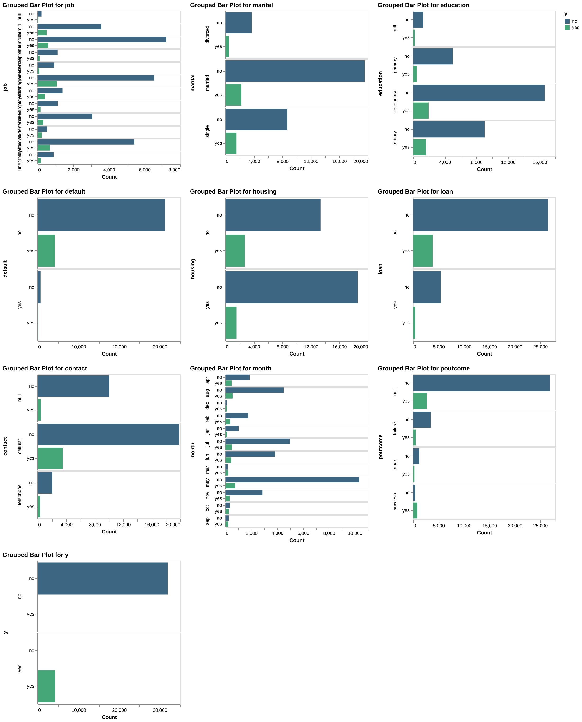
Fig. 1 Categorical variables.

Continuous variables

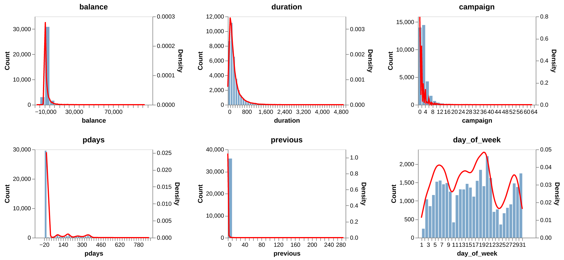
Fig. 2 Continuous variables.

Log continuous variables

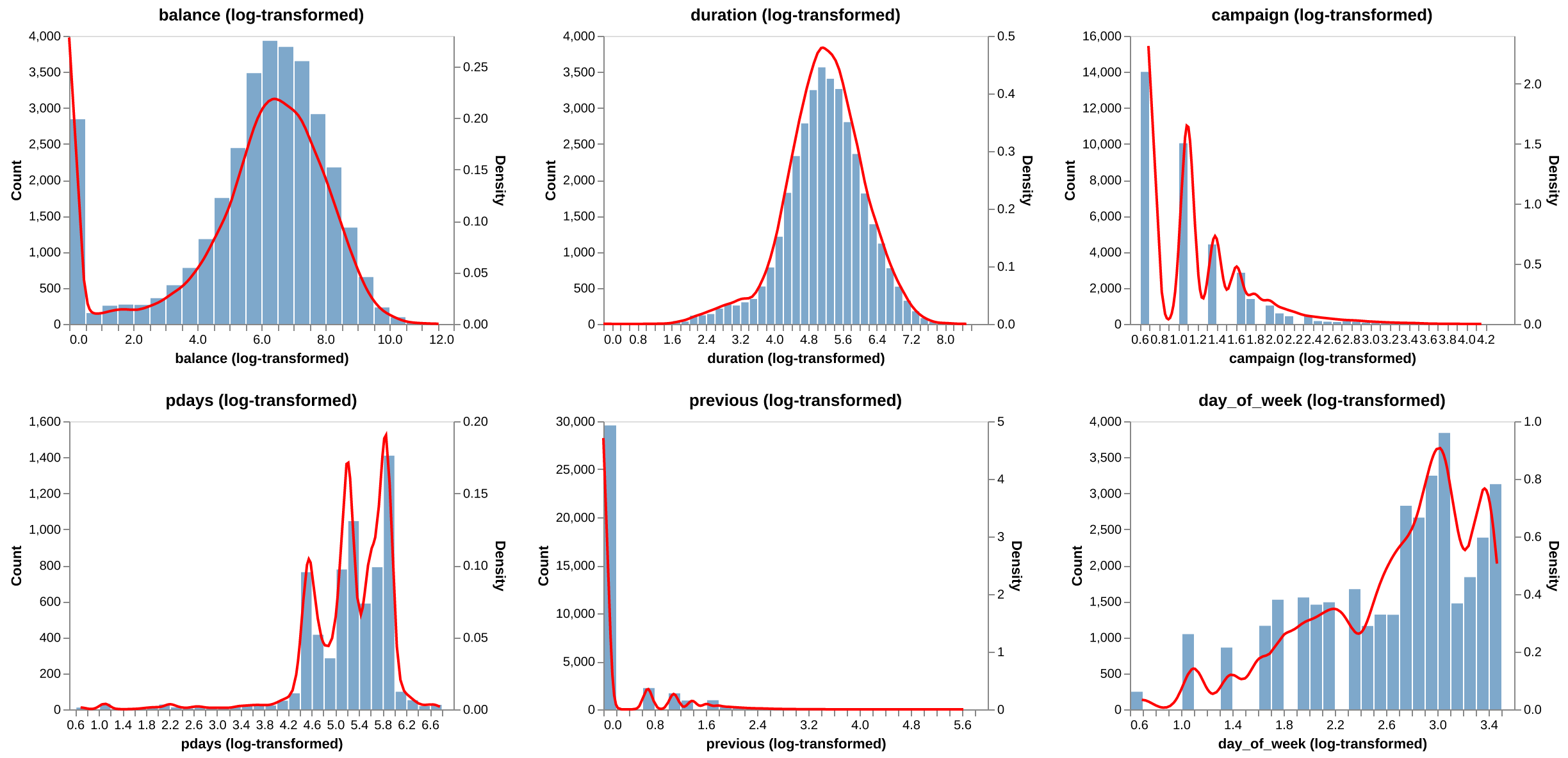
Fig. 3 Log continuous variables.

Data Preprocessing

Column Transformer

In this section, we have defined lists with the names of the features according to their type.

Then, we define all the transformations that have to be applied to the different columns. We define the order of the education levels as they belong to an ordinal variable and we create pipelines to manage nulls before each transformation. All of the transformations impute the most frequent value except for the numeric transformer, which imputes the median value.

Finally, we create a column transformer named preprocessor.

Resample

Because it is a class-imbalanced issue, we decided to utilize some resample technique to boost the performance of our model. reference: https://imbalanced-learn.org/stable/under_sampling.html

Modeling

1. Logistic Regression

First we applied a logistic regression model to our data. We used randomized search to find the best C parameter, as shown here (Figure 4):

Parameter	Value
C	0.626443

Fig. 4 Best parameter for the Logistic Regression model.

The best score generated by the model with the best parameter (Figure 5):

Metric	Value
Best Score	0.904371

Fig. 5 Best score for the Logistic Regression model.

Leveraging the logistic regression model with the best parameter, we got the below Receiver Operating Characteristic curve (Figure 6):

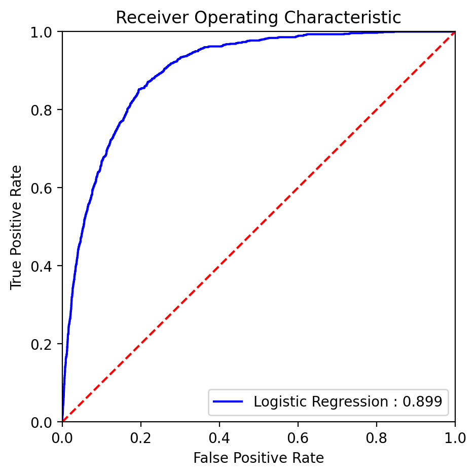
Fig. 6 ROC curve with AUC score for the Logistic Regression model.

The classification report (Figure 7):

	Precision	Recall	F1	Support
0	0.968	0.837	0.898	7985.000
1	0.392	0.793	0.524	1058.000
accuracy			0.832	9043.000
macro avg	0.680	0.815	0.711	9043.000
weighted avg	0.901	0.832	0.854	9043.000

Fig. 7 Classification report for the Logistic Regression model.

The precision, recall, F1, AUC (Figure 8):

Model	Recall	Precision	F1	AUC
Logistic Regression	0.793006	0.391690	0.524375	0.899340

Fig. 8 Key metrics for the Logistic Regression model.

And the confusion matrix (Figure 9):

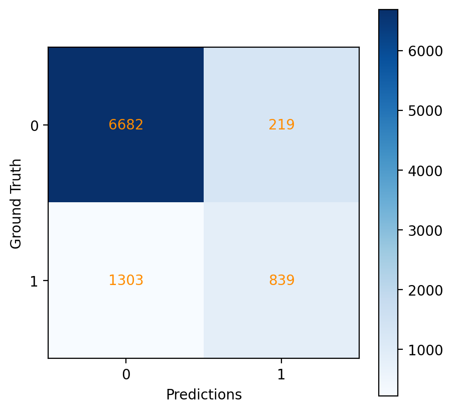
Fig. 9 Confusion matrix for the Logistic Regression model.

Discussion

The presented classification report provides a detailed evaluation of a model’s performance on a binary classification task. Here are some key observations:

Precision and Recall: Precision measures the accuracy of positive predictions, indicating that when the model predicts a positive outcome, it is correct approximately 39% of the time. Recall, on the other hand, suggests that the model successfully identifies around 79% of the actual positive cases.

F1-Score: The F1-Score is the harmonic mean of precision and recall, providing a balance between the two. In this case, it is calculated at approximately 52%, reflecting a moderate balance between precision and recall.

Accuracy: The overall accuracy of the model is 83%, indicating the percentage of correctly predicted instances among all instances.

Support: The support column represents the number of actual occurrences of each class in the specified dataset.

Macro and Weighted Averages: The macro average calculates the unweighted average of precision, recall, and F1-score across classes, while the weighted average considers the support of each class. The macro average of the F1-score is around 71%, and the weighted average is approximately 85%.

AUC: The AUC for the logistic regression model is noted as approximately 90%. This suggests the model’s strong capability in distinguishing between the classes.

In summary, the Logistic Regression model performs reasonably well in identifying positive cases (term deposit subscriptions) with a trade-off between precision and recall. The overall evaluation metrics provide insights into the model’s strengths and areas for potential improvement.

2. KNN

Then we implemented a KNN model on our dataset. To optimize the model, we still employed randomized search approach for determining the most effective parameters, n_neighbors and weights (Figure 10):

Parameter	Value
n_neighbors	34
weights	distance

Fig. 10 Best parameter for the KNN model.

The corresponding best score of the optimized KNN model (Figure 11):

Metric	Value
Best Score	0.898097

Fig. 11 Best score for the KNN model.

By utilizing the KNN model optimized with the best parameters, we obtained the following ROC curve (Figure 12):

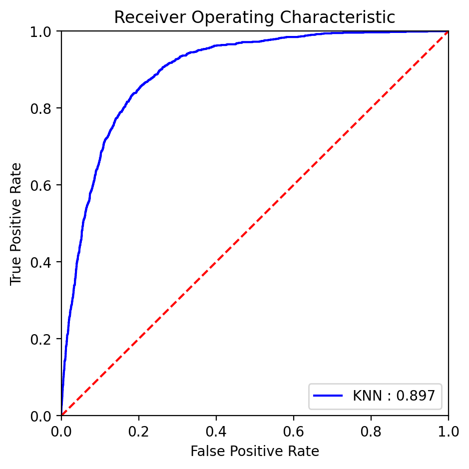
Fig. 12 ROC curve with AUC score for the KNN model.

The classification report (Figure 13):

	Precision	Recall	F1	Support
0	0.966	0.857	0.908	7985.0
1	0.418	0.774	0.543	1058.0
accuracy			0.848	9043.0
macro avg	0.692	0.816	0.726	9043.0
weighted avg	0.902	0.848	0.866	9043.0

Fig. 13 Classification report for the KNN model.

The precision, recall, F1, AUC (Figure 14):

Model	Recall	Precision	F1	AUC
KNN	0.774102	0.418070	0.542923	0.896745

Fig. 14 Key metrics for the KNN model.

And the confusion matrix (Figure 15):

Fig. 15 Confusion matrix for the KNN model.

Discussion

Based on the above results of the KNN model’s performance, we got some key findings:

Precision and Recall: For the positive class, the precision is about 42%, which indicates room for improvement in the accuracy of positive predictions. The positive class has a recall of approximately 77%, showing the model’s proficiency in detecting the actual positive instances.

F1-Score: For the positive class, the F1-score is around 54%, suggesting a moderate balance that could benefit from enhancement.

Accuracy: The model’s accuracy is reported at 85%, reflecting the proportion of correctly predicted instances out of all predictions made.

Support: The support metric indicates the actual occurrence of each class in the dataset, with 7985 instances for the negative class and 1058 for the positive class.

Macro and Weighted Averages: The macro average, which computes an unweighted mean across classes, presents an F1-score of approximately 73%, while the weighted average, taking into account the support for each class, is around 87%.

AUC: The AUC for the Decision Tree model is noted as approximately 90%

Summarizing the KNN model’s performance, it shows a strong ability in identifying negative cases with high precision and recall, while for positive cases, it demonstrates a fair detection rate with scope for improvement in precision.

3. Decision Tree

We now implemented a decision tree and conducted a randomized search to identify the optimal parameters. The results of the best parameters are depicted here (Figure 16):

Parameter	Value
max_depth	6
criterion	entropy

Fig. 16 Best parameter for the Decision Tree model.

With the best max_depth and criterion, we got the below best score (Figure 17):

Metric	Value
Best Score	0.876534

Fig. 17 Best score for the Decision Tree model.

Utilizing the logistic regression model with the optimal parameter, we generated the ROC curve presented below (Figure 18):

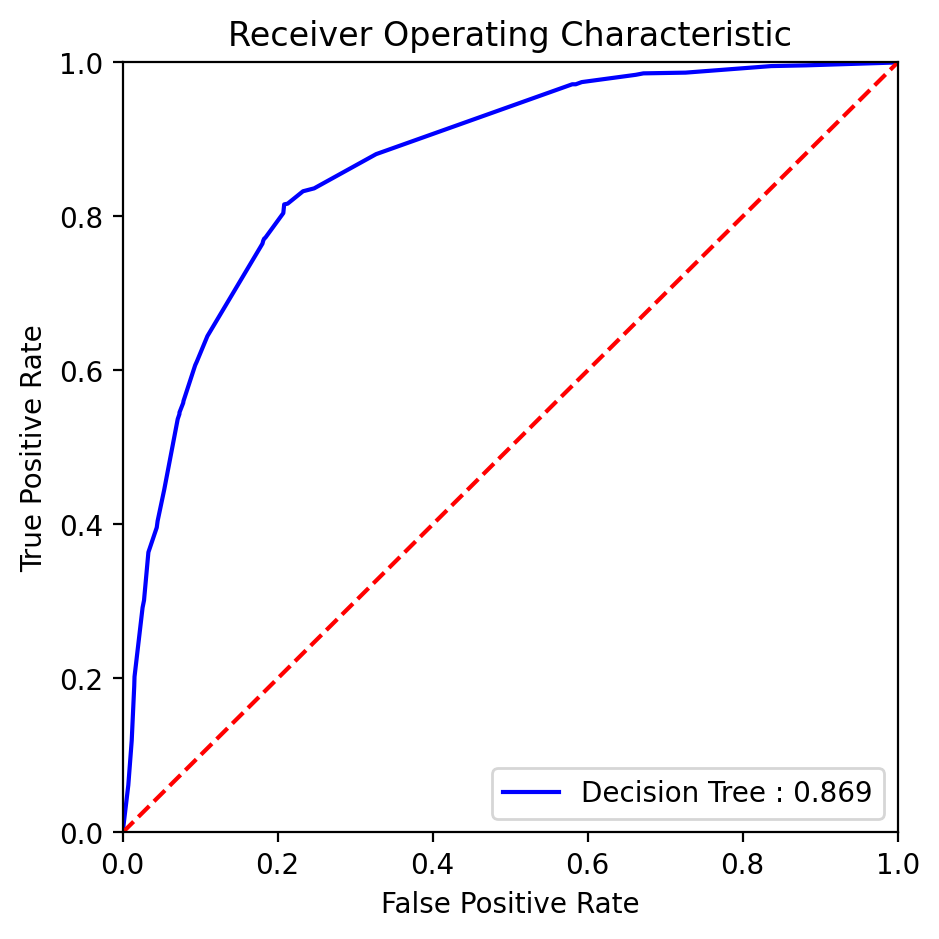
Fig. 18 ROC curve with AUC score for the Decision Tree model.

The classification report (Figure 19):

	Precision	Recall	F1	Support
0	0.97	0.792	0.872	7985.0
1	0.342	0.816	0.481	1058.0
accuracy			0.794	9043.0
macro avg	0.656	0.804	0.677	9043.0
weighted avg	0.897	0.794	0.826	9043.0

Fig. 19 Classification report for the Decision Tree model.

The precision, recall, F1, AUC (Figure 20):

Model	Recall	Precision	F1	AUC
Decision Tree	0.815690	0.341512	0.481450	0.868667

Fig. 20 Key metrics for the Decision Tree model.

And the confusion matrix (Figure 21):

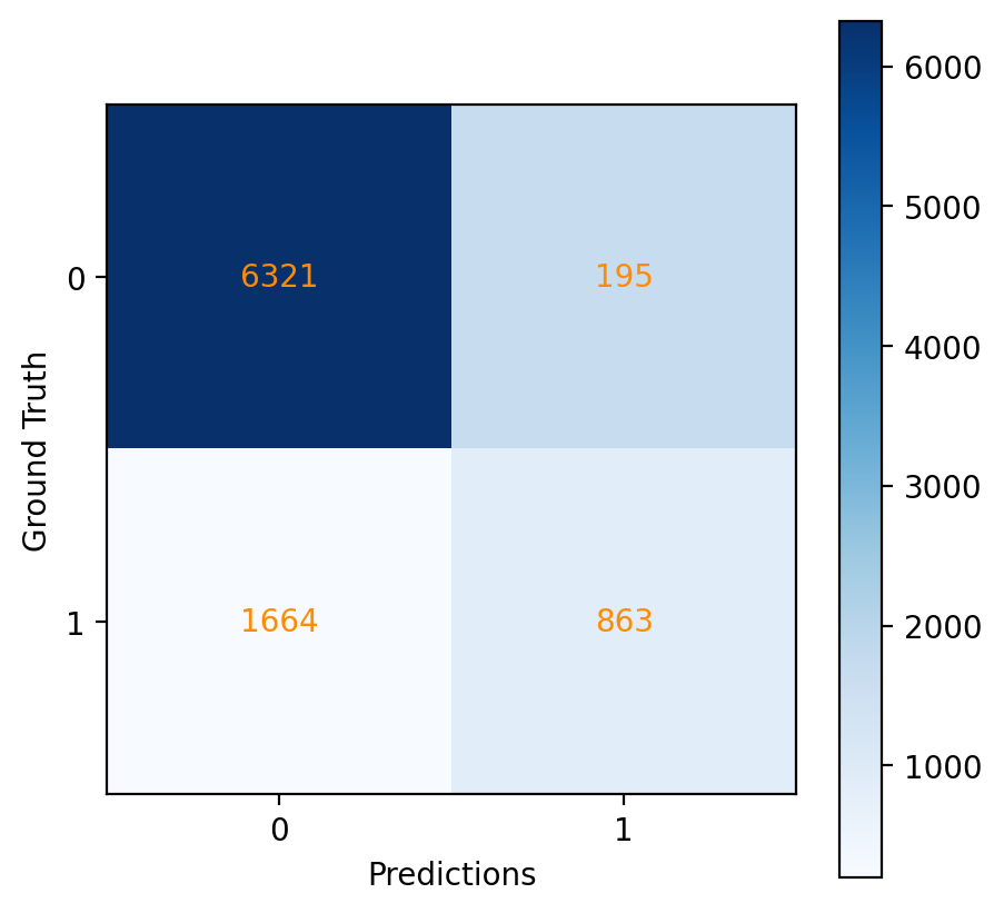
Fig. 21 Confusion matrix for the Decision Tree model.

Discussion

Some key observations for the above decision tree model:

Precision and Recall: For the positive class, precision drops significantly to around 34%, suggesting that positive predictions are less reliable. However, the recall for the positive class is high at approximately 82%, which means the model is adept at capturing most of the actual positive cases.

F1-Score: For the positive class, the F1-score is around 48%, indicating a moderate balance with potential room for improvement.

Accuracy: The accuracy of the Decision Tree model is calculated at approximately 79%, which reflects the percentage of correctly predicted instances among all instances.

Support: The ‘support’ metric denotes the actual number of occurrences for each class in the dataset, with 7985 instances for the negative class and 1058 instances for the positive class.

Macro and Weighted Averages: The macro average, which provides an unweighted mean of precision, recall, and F1-score across classes, is calculated at around 68%. The weighted average, which accounts for the support of each class, is approximately 83%.

AUC: The AUC for the Decision Tree model is noted as approximately 87%.

In summary, the Decision Tree model demonstrates a strong ability to identify negative cases, with excellent precision and a good recall rate. While it identifies positive cases with high recall, the precision for positive predictions is quite low, suggesting a significant area for improvement.

4. Naive Bayes

Finally we also tried a Naive Bayes model, and employed a randomized search to identify the most best parameters (Figure 22):

Parameter	Value
var_smoothing	0.126892

Fig. 22 Best parameter for the Naive Bayes model.

The best score generated by the model with the best parameter (Figure 23):

Metric	Value
Best Score	0.844517

Fig. 23 Best score for the Naive Bayes model.

Utilizing the Naive Bayes model fine-tuned with the optimal parameter, we generated the following ROC curve (Figure 24):

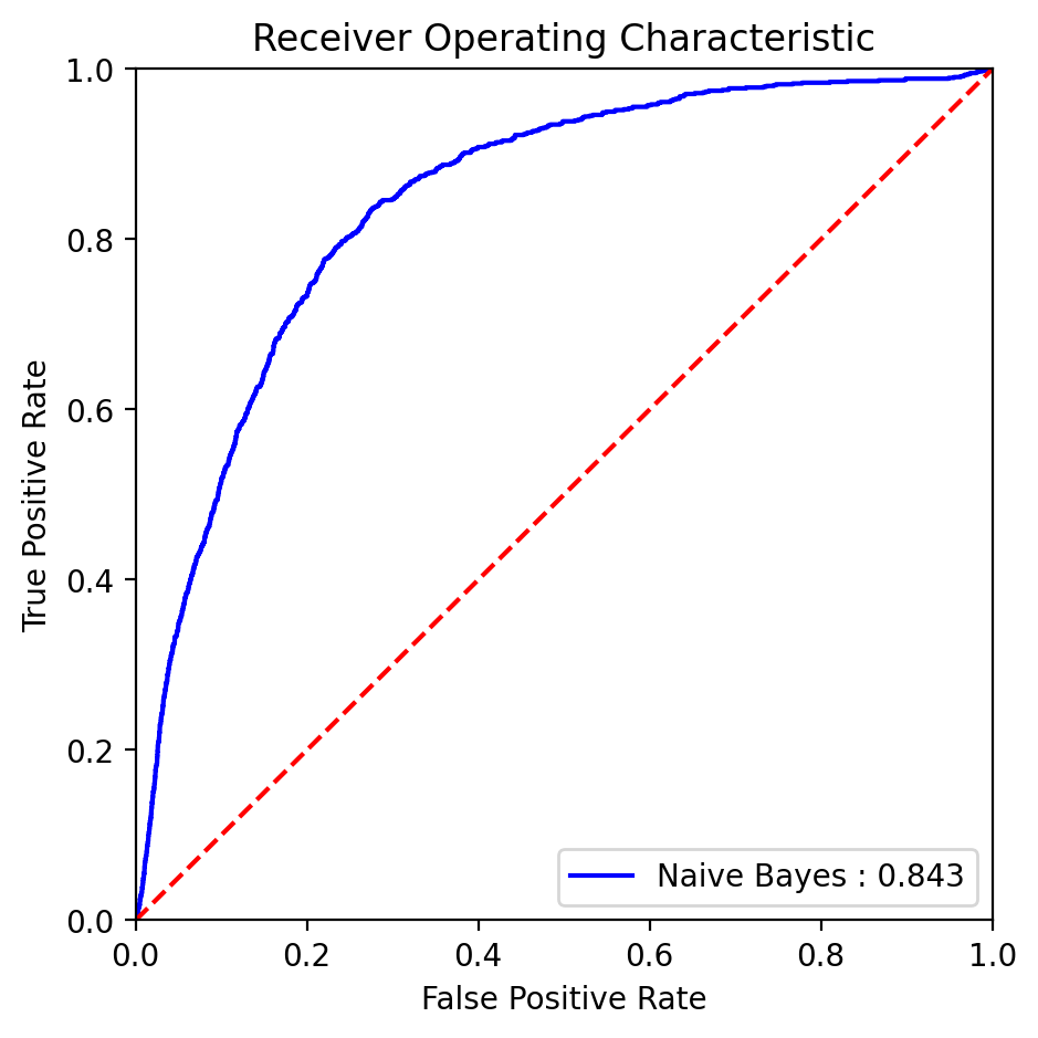
Fig. 24 ROC curve with AUC score for the Naive Bayes model.

The classification report (Figure 25):

	Precision	Recall	F1	Support
0	0.935	0.892	0.913	7985.0
1	0.397	0.535	0.456	1058.0
accuracy			0.850	9043.0
macro avg	0.666	0.714	0.685	9043.0
weighted avg	0.872	0.85	0.860	9043.0

Fig. 25 Classification report for the Naive Bayes model.

The precision, recall, F1, AUC (Figure 26):

Model	Recall	Precision	F1	AUC
Naive Bayes	0.534972	0.396914	0.455717	0.842733

Fig. 26 Key metrics for the Naive Bayes model.

And the confusion matrix (Figure 27):

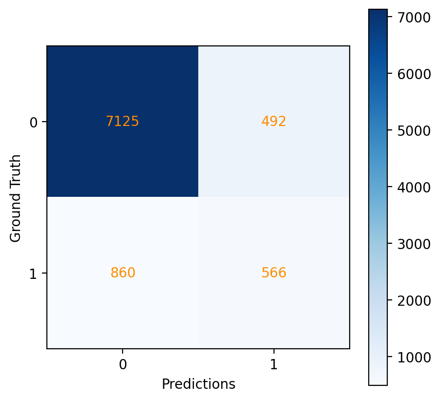
Fig. 27 Confusion matrix for the Naive Bayes model.

Discussion

Findings from the evaluation of the Naive Bayes model’s performance:

Precision and Recall: For the positive class, the precision is significantly lower, at about 40%, showing that positive predictions are correct less than half of the time. The recall for the positive class is about 54%, indicating that the model is moderately effective at identifying actual positive cases.

F1-Score: For the positive class, the F1-score is about 46%, which indicates that there is room for improvement in balancing precision and recall for the positive predictions.

Accuracy: The model’s overall accuracy is 85%, reflecting the proportion of correctly predicted instances out of all predictions made.

Support: The ‘support’ value indicates the actual number of instances for each class in the dataset, with 7985 instances for the negative class and 1058 instances for the positive class.

Macro and Weighted Averages: The macro average, which calculates an unweighted mean of precision, recall, and F1-score across both classes, is around 68%. The weighted average, which accounts for the class distribution (support), is approximately 86%.

AUC: The Naive Bayes model has an AUC of approximately 84%.

In summary, the Naive Bayes model performs very well in identifying negative cases with high precision and recall, while it shows moderate effectiveness in identifying positive cases. The overall accuracy is quite high, and the AUC indicates a good discriminative ability. The model shows a strong performance on the negative class but there is a notable discrepancy in the positive class predictions, where both precision and recall could be improved for better balance and performance.

Model Comparison

Aggregated Results

We plotted the ROC curves for various models on a single graph (Figure 28) and combined the scores into one table for comparison (Figure 29):

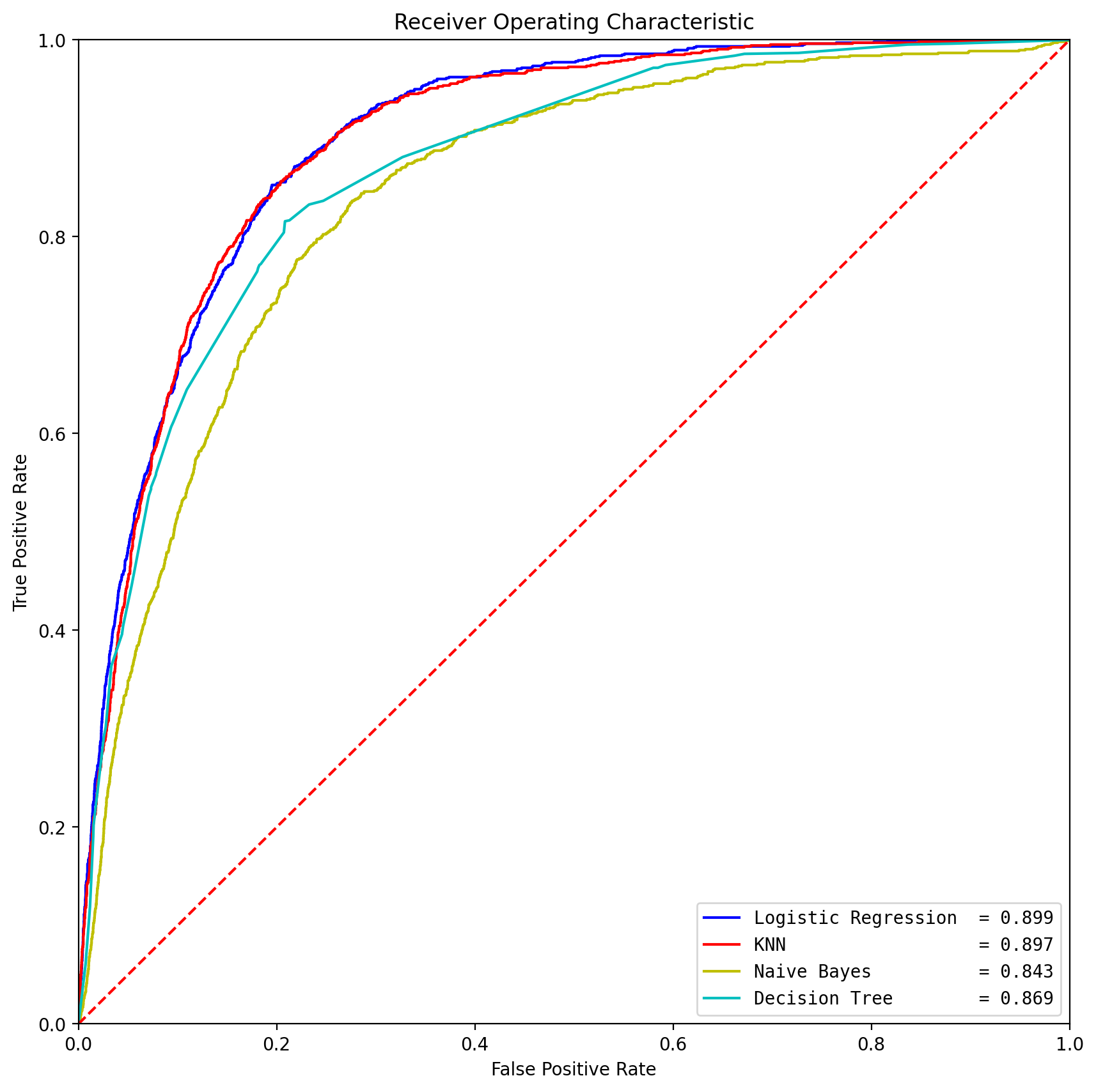
Fig. 28 ROC for all the tested models.

Model	Recall	Precision	F1	AUC
Logistic Regression	0.793006	0.391690	0.524375	0.899340
KNN	0.774102	0.418070	0.542923	0.896745
Decision Tree	0.815690	0.341512	0.481450	0.868667
Naive Bayes	0.534972	0.396914	0.455717	0.842733

Fig. 29 Metrics comparison for all the tested models.

Comparison of Models

The table provides an overview of key evaluation metrics for different machine learning models applied to a binary classification task, specifically predicting customer subscription to a term deposit in a bank’s telemarketing campaign. Let’s analyze each metric for each model:

Logistic Regression

Recall Score (Sensitivity): 79% indicates the model’s ability to identify actual positive cases, capturing a substantial portion of them. Precision: 39% reflects the accuracy of positive predictions, indicating that when the model predicts a positive outcome, it is correct about 39% of the time. F1-Score: 52% is the harmonic mean of precision and recall, providing a balanced measure, though still moderate. Area Under the Curve (AUC): 90% signifies the model’s overall ability to distinguish between positive and negative instances.

KNN (K-Nearest Neighbors)

Recall Score (Sensitivity): 77% indicates the model’s effectiveness in capturing actual positive cases. Precision: 42% reflects the accuracy of positive predictions. F1-Score: 54% is the harmonic mean of precision and recall, showing a moderate balance. AUC: 90% signifies good overall discriminative ability.

Decision Tree

Recall Score (Sensitivity): 82% indicates a high ability to capture actual positive cases. Precision: 34% reflects the accuracy of positive predictions, but it’s lower compared to other models. F1-Score: 48% is the harmonic mean of precision and recall, showing a moderate balance. AUC: 87% indicates a good ability to distinguish between positive and negative instances.

Naive Bayes

Recall Score (Sensitivity): 53% indicates a moderate ability to capture actual positive cases. Precision: 40% reflects the accuracy of positive predictions. F1-Score: 46% is the harmonic mean of precision and recall, showing a moderate balance. AUC: 84% suggests a reasonable ability to discriminate between positive and negative instances.

In summary, the models show varying performance across metrics, while Logisitic Regression shows the best performance.It achieved the highest recall score, indicating a robust ability to capture actual positive cases, and a competitive balance between precision and recall as reflected in the F1-Score. Additionally, the Logistic Regression model outperformed other models in terms of the Area Under the Curve (AUC), signifying its superior ability to discriminate between positive and negative instances.

Feature Importance

Finally, we chose Logistic Regression model and analysed the key features as determined by the model for predicting whether a client will subscribe to a term deposit.

The importance of the key features are demonstrated below (Figure 30):

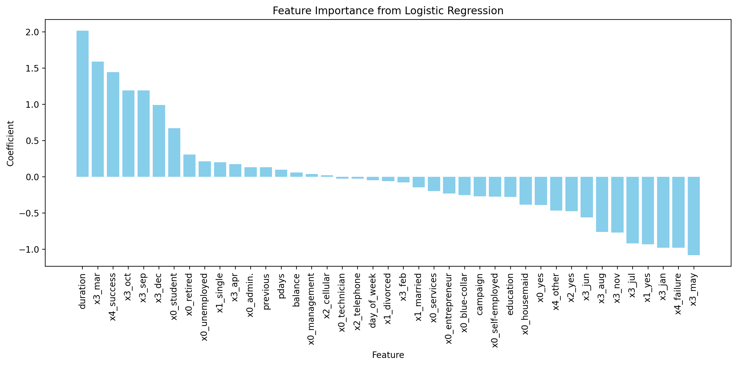
Fig. 30 Feature importance for the Logistic Regression model.

The analysis of key features from the logistic regression model provides significant insights into the factors that influence a client’s decision to subscribe to a term deposit. The most influential feature appears to be the ‘duration’ of the last contact, which is intuitive as longer conversations might indicate a higher interest level in the product being offered. Following closely are categorical variables related to the last contact month (‘x3_mar’, ‘x3_sep’, etc.), suggesting that the timing of the contact can substantially affect the outcome, possibly due to seasonal financial behavior or marketing campaign effectiveness.

Job roles also play a critical role, with ‘x0_student’ and ‘x0_retired’ featuring prominently, which might reflect different financial needs or availabilities of these demographic groups. Interestingly, marital status (‘x0_single’) and success of previous campaigns (‘x3_success’) are also important, highlighting that personal circumstances and past interactions with the bank can sway a client’s decision.

On the other end of the spectrum, the negative coefficients associated with certain months (‘x3_jan’, ‘x3_jul’, ‘x3_may’) and the ‘x4_failure’ variable, which represents the outcome of the previous campaign, indicate a decreased likelihood of a subscription. This suggests that unsuccessful prior marketing efforts or certain times of the year might be less opportune for initiating term deposit subscriptions.

Conclusion

Our analysis suggests that the logistic regression model performs robustly in predicting whether clients will subscribe to a term deposit in a Portuguese banking institution context. The ROC curve illustrates that logistic regression, with an AUC of 90%, provides a superior balance between true positive rate and false positive rate compared to other models like KNN, Naive Bayes, and Decision Trees. This high AUC value indicates that logistic regression has a high ability to distinguish between those clients who will subscribe and those who will not.

The feature importance graph from the logistic regression model reveals that certain features such as the duration of the last contact, the month of the last contact, and certain job roles are highly influential in predicting subscription outcomes. Features with positive coefficients like ‘duration’, ‘x3_mar’ (March), and ‘x4_success’ (previous campaign success) suggest these aspects enhance the likelihood of a client subscribing to a term deposit. Conversely, features such as ‘x3_may’ (May) and ‘x4_failure’ (previous campaign failure) are negatively correlated with the subscription likelihood, indicating potential areas for marketing strategy improvement.

However, the assumptions inherent in logistic regression may affect our conclusions. Logistic regression assumes a linear relationship between the log-odds of the dependent variable and each independent variable. This may not capture complex relationships in the data, and certain influential interactions between features could be overlooked. Furthermore, logistic regression assumes that the observations are independent of each other, which may not be the case in a marketing campaign where clients could be influenced by external factors or by each other. Considering these limitations, we will further improve our analysis when applying our findings to real-world scenarios.

Useful Links

Github repo url: UBC-MDS/bank-marketing-analysis
Release url: https://ubc-mds.github.io/bank-marketing-analysis

References

DFH+15

Cynthia Dwork, Vitaly Feldman, Moritz Hardt, Toni Pitassi, Omer Reingold, and Aaron Roth. Generalization in adaptive data analysis and holdout reuse. Advances in Neural Information Processing Systems, 2015.

FK15

Peter Flach and Meelis Kull. Precision-recall-gain curves: pr analysis done right. Advances in neural information processing systems, 2015.

MRC12

S. Moro, P. Rita, and P. Cortez. Bank Marketing. UCI Machine Learning Repository, 2012. DOI: https://doi.org/10.24432/C5K306.

MCR14

Sérgio Moro, Paulo Cortez, and Paulo Rita. A data-driven approach to predict the success of bank telemarketing. Decision Support Systems, 62:22–31, 2014.