What is Supervised Machine Learning?

Prevalence of Machine Learning (ML)

You may not know it, but machine learning (ML) is all around you.

Some examples include:

• Voice assistance
• Google news
• Recommender systems
• Face recognition
• Auto completion
• Stock market predictions
• Character recognition
• Self-driving cars
• Cancer diagnosis
• Drug discovery

The best AlphaGo player in the world is not human anymore.

AlphaGo, a machine learning-based system from Google, is the world’s best player at the moment.

What is Machine Learning?

• A field of study that gives computers the ability to learn without being explicitly programmed.*
  – Arthur Samuel (1959)

What exactly is machine learning? There is no clear consensus on the definition of machine learning. But here is a popular definition by Artur Samuel who was one of the pioneers of machine learning and artificial intelligence.

Arthur Samuel said that machine learning is “A field of study that gives computers the ability to learn without being explicitly programmed.”

Machine learning is a different way to think about problem-solving. Usually, when we write a program we’re thinking logically and mathematically. Here is how a traditional program looks like. We are given input and an algorithm and we produce an output.

Instead, in the machine learning paradigm, we’re given data and some output and our machine learning algorithm returns a program. we can use this program to predict the output for some unseen input.

In this paradigm, we’re making observations about an uncertain world and thinking about it statistically.

Some concrete examples of supervised learning

Example 1: Predict whether a patient has a liver disease or not

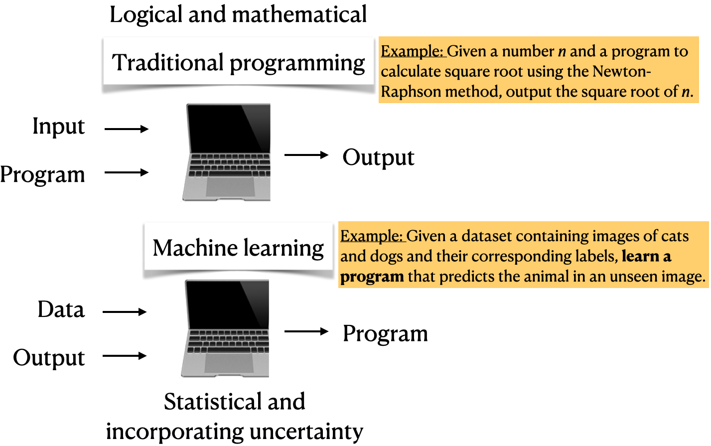
In all the the upcoming examples, Don’t worry about the code. Just focus on the input and output in each example.

Before we start let’s look at some concrete examples of supervised machine learning.

Our first example is predicting whether a patient has a liver disease or not.

For now, ignore the code and only focus on input and output.

train_df, test_df = train_test_split(df, test_size=4, random_state=16)
train_df.head()

	Age	Total_Bilirubin	Direct_Bilirubin	Alkaline_Phosphotase	...	Total_Protiens	Albumin	Albumin_and_Globulin_Ratio	Target
13	74	1.1	0.4	214	...	8.1	4.1	1.0	1
236	22	0.8	0.2	300	...	7.9	3.8	0.9	0
335	13	0.7	0.1	182	...	8.9	4.9	1.2	1
234	40	0.9	0.2	285	...	7.7	3.5	0.8	1
159	50	1.2	0.4	282	...	7.2	3.9	1.1	1

5 rows × 10 columns

Usually, for supervised machine learning, we are provided data in a tabular form.

We have columns full of data and a special “target” column which is what we are trying to predict.

We pass this to a machine learning algorithm.

from xgboost import XGBClassifier
X_train = train_df.drop(columns=['Target'])
y_train = train_df['Target']
X_test = test_df.drop(columns=['Target'])
model = XGBClassifier()
model.fit(X_train, y_train);

Next, we build a model and train our model using the labels we already have.

Ignore this output here.

It’s just explaining what’s going on in the model which we will explain soon.

pred_df = pd.DataFrame(
    {"Predicted label": model.predict(X_test).tolist()}
)
df_concat = pd.concat([X_test.reset_index(drop=True), pred_df], axis=1)
df_concat

	Age	Total_Bilirubin	Direct_Bilirubin	Alkaline_Phosphotase	...	Total_Protiens	Albumin	Albumin_and_Globulin_Ratio	Predicted label
0	61	0.7	0.2	145	...	5.8	2.7	0.87	0
1	42	11.1	6.1	214	...	6.9	2.8	2.80	1
2	22	0.8	0.2	198	...	6.8	3.9	1.30	0
3	72	1.7	0.8	200	...	6.2	3.0	0.93	1

4 rows × 10 columns

Then, given new unseen input, we can apply our learned model to predict the target for the input.

In this case, we can imagine that a new patient arrives and we want to predict if the patient has a disease or not.

Given the patient’s information, our model predicts if the patient has the disease or not.

Example 2: Predict the label of a given image

Our second example is predicting the label of a given image.

Predict labels with associated probability scores for unseen images

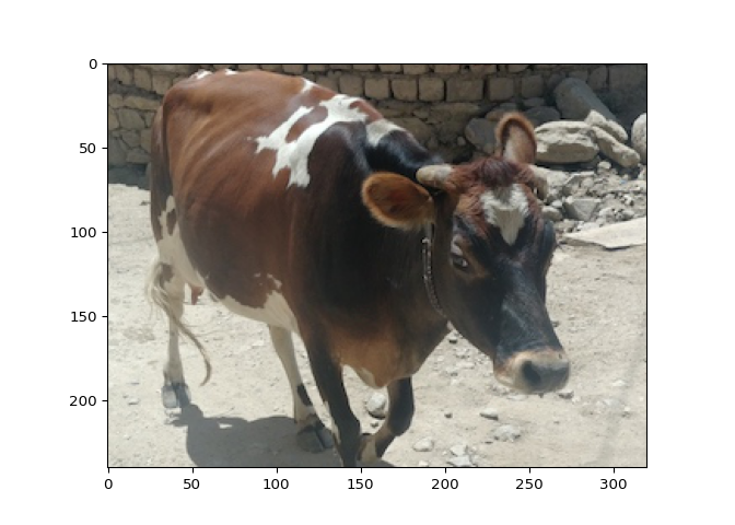
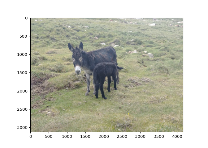
images = glob.glob("test_images/*.*")
for image in images:
    img = Image.open(image)
    img.load()
    plt.imshow(img)
    plt.show()
    df = classify_image(img)
    print(df.to_string(index=False))

  Class  Probability
      ox     0.869893
  oxcart     0.065034
  sorrel     0.028593
 gazelle     0.010053

Here we use a machine learning model trained on millions of images and their labels.

We are applying our model to predict the labels of unseen images.

In this particular case, our unseen image is that of an ox.

When we apply our trained model on this image, it gives us some predictions and their associated probability scores.

So in this particular case, the model predicted that the image was that of an ox with a confidence of 0.869.

images = glob.glob("test_images/*.*")
for image in images:
    img = Image.open(image)
    img.load()
    plt.imshow(img)
    plt.show()
    df = classify_image(img)
    print(df.to_string(index=False))

            Class  Probability
            llama     0.123625
               ox     0.076333
           kelpie     0.071548
 ibex, Capra ibex     0.060569

Our second unseen image contains some donkeys.

In this case, when we apply our mode to the image, The model predicts that it contains a llama. That being said, the probability score here is only 0.123.

Example 3: Predict sentiment expressed in a movie review (pos/neg)

Attribution: The dataset imdb_master.csv was obtained from Kaggle and downsampled for demonstration

Our third example is about predicting sentiment expressed in movie reviews.

train_df.head()

	review	label
684	as i said in the other comment this is one of ...	pos
916	David Webb Peoples meets Paul Anderson...if it...	pos
701	Some people don't like Led Zeppelin, but lucki...	pos
560	Russian emigrant director in Hollywood in 1928...	pos
795	At least it is with this episode. Here we have...	neg

First we wrangle our data so that we can train our model.

This data contains the review in a column named review and a label column which contains values of either pos or neg for positive or negative.

X_train, y_train = train_df['review'], train_df['label']
X_test, y_test = test_df['review'], test_df['label']

clf = Pipeline(
    [
        ("vect", CountVectorizer(max_features=5000)),
        ("clf", LogisticRegression(max_iter=5000)),
    ]
)
clf.fit(X_train, y_train);

Next, we build our model and train on our existing data.

Again, don’t worry about the code here.

pred_dict = {
    "reviews": X_test[0:4],
    "true_sentiment": y_test[0:4],
    "sentiment_predictions": clf.predict(X_test[0:4]),
}
pred_df = pd.DataFrame(pred_dict)
pred_df.head()

	reviews	true_sentiment	sentiment_predictions
953	By submitting this comment you are agreeing to...	pos	pos
770	Kinda funny how comments for this film went co...	neg	neg
336	It is a story as old as man. The jealousy for ...	neg	neg
87	Perhaps once in a generation a film comes alon...	pos	pos

Once we have the model, we can use this to predict the sentiment expressed in new movie reviews.

Example 4: Predict housing prices

Attribution: The dataset kc_house_data.csv was obtained from Kaggle and downsampled for demonstration.

Example 4 is about predicting housing prices.

df = pd.read_csv("data/kc_house_data.csv")
train_df, test_df = train_test_split(df, test_size=0.2, random_state=4)
train_df.head()

	price	bedrooms	bathrooms	sqft_living	...	lat	long	sqft_living15	sqft_lot15
608	219000.0	3	1.50	1740	...	47.3657	-122.094	1540	5200
511	618250.0	4	3.25	2520	...	47.6801	-122.315	1730	3360
641	200000.0	2	1.50	1360	...	47.2852	-122.190	1360	1898
112	656500.0	4	2.00	2710	...	47.6756	-122.305	1700	3800
535	530000.0	3	1.75	1660	...	47.5734	-122.412	1510	4800

5 rows × 19 columns

In this particular case, our data contains attributes associated with properties

For example, our attributes consist of the number of bedrooms, the number of bathrooms, etc.

Our special column which we call our “target column” is the price for the corresponding property.

Note that this price column here contains continuous values and not discrete values as we saw in our previous examples.

X_train = train_df.drop(columns=["price"])
X_train.head()

	bedrooms	bathrooms	sqft_living	sqft_lot	...	lat	long	sqft_living15	sqft_lot15
608	3	1.50	1740	5200	...	47.3657	-122.094	1540	5200
511	4	3.25	2520	3360	...	47.6801	-122.315	1730	3360
641	2	1.50	1360	1898	...	47.2852	-122.190	1360	1898
112	4	2.00	2710	4750	...	47.6756	-122.305	1700	3800
535	3	1.75	1660	4800	...	47.5734	-122.412	1510	4800

5 rows × 18 columns

y_train = train_df["price"]
y_train.head()

608    219000.0
511    618250.0
641    200000.0
112    656500.0
535    530000.0
Name: price, dtype: float64

X_test = test_df.drop(columns=["price"])
y_test = train_df["price"]

It’s important that we separate our data from the target column (The y variables).

from xgboost import XGBRegressor

model = XGBRegressor()
model.fit(X_train, y_train);

Again we use this data to train our machine learning model.

pred_df = pd.DataFrame(
    {"Predicted price": model.predict(X_test[0:4]).tolist(), "Actual price": y_test[0:4].tolist()}
)
df_concat = pd.concat([X_test[0:4].reset_index(drop=True), pred_df], axis=1)
df_concat.head()

	bedrooms	bathrooms	sqft_living	sqft_lot	...	sqft_living15	sqft_lot15	Predicted price	Actual price
0	3	2.25	1400	6970	...	1800	8140	383849.40625	219000.0
1	4	2.50	3440	6332	...	3310	6528	853539.31250	618250.0
2	5	2.00	2330	10750	...	1830	10180	414617.37500	200000.0
3	3	1.75	1840	2310	...	1670	4000	781376.31250	656500.0

4 rows × 20 columns

And once we have our trained model, we apply it to predict the price associated with new home properties.

When we pass new properties into the model we get a predicted price for those properties.

And note again that our predicted prices here are continuous numbers and not discrete values

Let’s apply what we learned!