𝑘 -Nearest Neighbours Regressor

Regression with 𝑘-nearest neighbours ( 𝑘 -NNs)

np.random.seed(0)
n = 50
X_1 = np.linspace(0,2,n)+np.random.randn(n)*0.01
X = pd.DataFrame(X_1[:,None], columns=['length'])
X.head()

	length
0	0.017641
1	0.044818
2	0.091420
3	0.144858
4	0.181941

y = abs(np.random.randn(n,1))*2 + X_1[:,None]*5
y = pd.DataFrame(y, columns=['weight'])
y.head()

	weight
0	1.879136
1	0.997894
2	1.478710
3	3.085554
4	0.966069

We can use the 𝑘-nearest neighbour algorithm on regression problems as well.

In 𝑘-nearest neighbour regression, we take the average of 𝑘-nearest neighbours instead of majority vote.

Let’s look at an example. Here we are creating some synthetic data with fifty examples and only one feature.

Let’s imagine that our one feature represents the length of a snake and our task is to predict the weight of the snake given the length.

Right now, do not worry about the code and only focus on data and our model.

X_train, X_test, y_train, y_test = train_test_split(X, y, test_size=0.2, random_state=123)

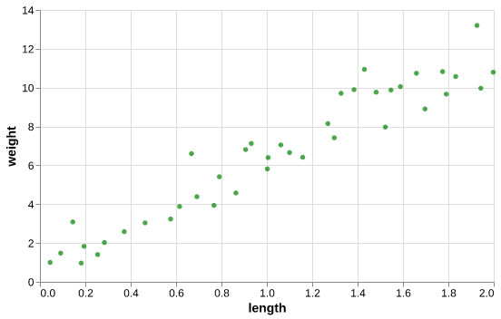
import altair as alt
source = pd.concat([X_train, y_train], axis=1)

scatter = alt.Chart(source, width=500, height=300).mark_point(filled=True, color='green').encode(
    alt.X('length:Q'),
    alt.Y('weight:Q'))

scatter

Let’s split over data first so there we do not break the golden rule of machine learning.

And here is what our data looks like.

We only have one feature of length and our goal is to predict weight.

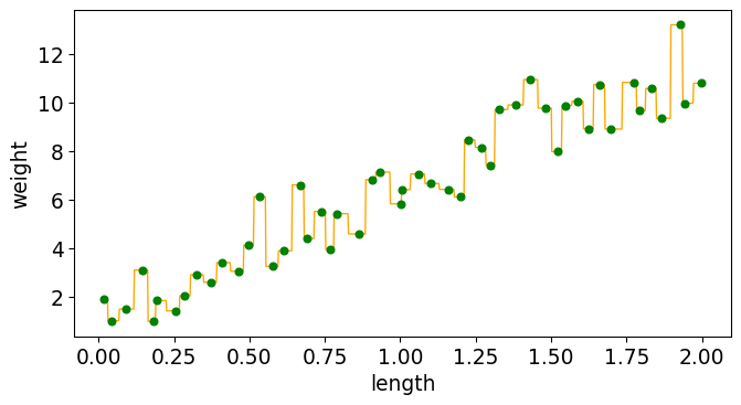
from sklearn.neighbors import KNeighborsRegressor

knnr = KNeighborsRegressor(n_neighbors=1, weights="uniform")
knnr.fit(X_train,y_train);

predicted = knnr.predict(X_train)
predicted[:5]

array([[ 4.57636104],
       [13.20245224],
       [ 3.03671796],
       [10.74123618],
       [ 1.82820801]])

knnr.score( X_train, y_train)  

1.0

Now let’s try the 𝑘-nearest neighbours regressor on this data.

In this case, we import KNeighborsRegressor instead of KNeighborsClassifier.

Then we create our KNeighborsRegressor object with n_neighbors=1 so we are only considering 1 neighbour and with uniform weights.

We fit our model and predict on X_train.

Here are the first five predictions.

As expected we get continuous values as predictions.

If we scored over regressors we get this perfect score of one.

Now remember that we are using a n_neighbors=1, so we are likely to overfit.

Here is how our model would look like if we plotted it.

The model is trying to get every example correct since n_neighbors=1.

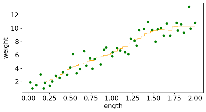
knnr = KNeighborsRegressor(n_neighbors=10, weights="uniform")
knnr.fit(X_train, y_train);

knnr.score(X_train, y_train)

0.9254540554756747

Now let’s try n_neighbors=10.

Again, we are creating our KNeighborsRegressor object with n_neighbors=10 and n_neighbors=10=’uniform’ which means all of our examples have equal contribution to the prediction.

We fit our regressor and score it. Now we can see we are getting a lower score over the training set. Our score decreased from 1.0 when to had n_neighbors=1 to now having a score of 0.932.

When we plot our model, we can see that it no longer is trying to get every example correct.

Using weighted distances

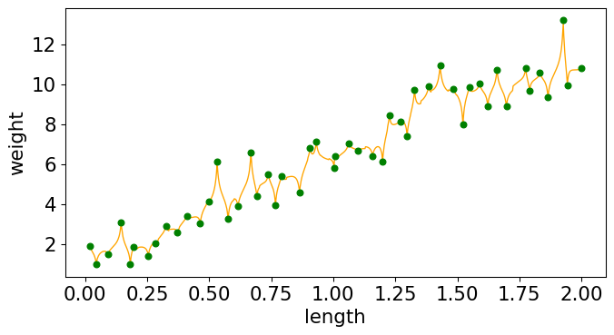
knnr = KNeighborsRegressor(n_neighbors=10, weights="distance")
knnr.fit(X_train, y_train);

knnr.score(X_train, y_train)

1.0

Let’s now take a look at the weight hyperparameter distance.

This means that the points (examples) that are closer now have more meaning to the prediction than the points (example) that are further away.

If we use this parameter, fit it and then score it, we get a perfect training score again.

Plotting it shows that the model is trying to predict every model correctly. This is likely another situation of overfitting.

Pros and Cons of 𝑘 -Nearest Neighbours

Pros:

• Easy to understand, interpret.
• Simply hyperparameter 𝑘 (n_neighbors) controlling the fundamental tradeoff.
• Can learn very complex functions given enough data.
• Lazy learning: Takes no time to fit

Cons:

• Can potentially be VERY slow during prediction time.
• Often not that great test accuracy compared to the modern approaches.
• You should scale your features. We’ll be looking into it in the next lecture.

Let’s talk about some pros and cons.

Advantages include:

• Easy to understand and interpret.
• Simply hyperparameter 𝑘 (n_neighbors) controlling the fundamental trade-off.
  • lower 𝑘 is likely producing an overfit model and higher 𝑘 is likely producing an underfit model.
• Given the simplicity of this algorithm, it can surprisingly learn very complex functions given enough data.
• 𝑘-Nearest Neighbours we don’t really do anything during the fit phase.

Some disadvantages often include:

• Can potentially be quite slow during prediction time which is due to the fact that it does very little during training time. During prediction, the model must find the distances to the query point to all examples in the training set and this makes it very slow.
• Scaling must be done when using this model, which will be covered in module 5.

Let’s apply what we learned!