cc_df = pd.read_csv('data/creditcard.csv.zip', encoding='latin-1')
train_df, test_df = train_test_split(cc_df, test_size=0.3, random_state=111)Introducing Evaluation Metrics
| Time | V1 | V2 | V3 | ... | V27 | V28 | Amount | Class | |
|---|---|---|---|---|---|---|---|---|---|
| 64454 | 51150.0 | -3.538816 | 3.481893 | -1.827130 | ... | -0.023636 | -0.454966 | 1.00 | 0 |
| 37906 | 39163.0 | -0.363913 | 0.853399 | 1.648195 | ... | -0.186814 | -0.257103 | 18.49 | 0 |
| 79378 | 57994.0 | 1.193021 | -0.136714 | 0.622612 | ... | -0.036764 | 0.015039 | 23.74 | 0 |
| 245686 | 152859.0 | 1.604032 | -0.808208 | -1.594982 | ... | 0.005387 | -0.057296 | 156.52 | 0 |
| 60943 | 49575.0 | -2.669614 | -2.734385 | 0.662450 | ... | 0.388023 | 0.161782 | 57.50 | 0 |
5 rows × 31 columns
| Time | V1 | V2 | V3 | ... | V27 | V28 | Amount | Class | |
|---|---|---|---|---|---|---|---|---|---|
| count | 199364.000000 | 199364.000000 | 199364.000000 | 199364.000000 | ... | 199364.000000 | 199364.000000 | 199364.000000 | 199364.000000 |
| mean | 94888.815669 | 0.000492 | -0.000726 | 0.000927 | ... | -0.000366 | 0.000227 | 88.164679 | 0.001700 |
| std | 47491.435489 | 1.959870 | 1.645519 | 1.505335 | ... | 0.401541 | 0.333139 | 238.925768 | 0.041201 |
| min | 0.000000 | -56.407510 | -72.715728 | -31.813586 | ... | -22.565679 | -11.710896 | 0.000000 | 0.000000 |
| 50% | 84772.500000 | 0.018854 | 0.065463 | 0.179080 | ... | 0.001239 | 0.011234 | 22.000000 | 0.000000 |
| max | 172792.000000 | 2.451888 | 22.057729 | 9.382558 | ... | 12.152401 | 33.847808 | 11898.090000 | 1.000000 |
6 rows × 31 columns
Baseline
from sklearn.dummy import DummyClassifier
from sklearn.model_selection import cross_validate

dummy = DummyClassifier(strategy="most_frequent")
pd.DataFrame(cross_validate(dummy, X_train, y_train, return_train_score=True)).mean()
fit_time 0.010974
score_time 0.000922
test_score 0.998302
train_score 0.998302
dtype: float64What is “positive” and “negative”?
Class
0    0.9983
1    0.0017
Name: proportion, dtype: float64There are two kinds of binary classification problems:
- Distinguishing between two classes
- Spotting a class (fraud transaction, spam, disease)
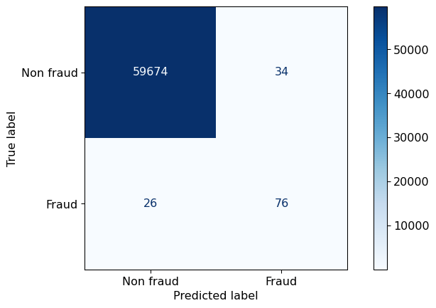
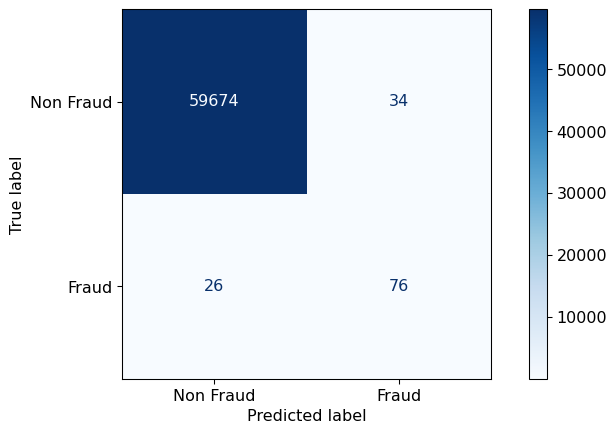
Confusion Matrix
| X | predict negative | predict positive |
|---|---|---|
| negative example | True negative (TN) | False positive (FP) |
| positive example | False negative (FN) | True positive (TP) |