Project Report¶

Salary predictor for tech employees in Canada based on survey data¶

Summary¶

Here we attempt to build the model to predict the income of tech employees in Canada by using a multi-linear regression model based on the following features: years of coding experience, programming languages used, education level, and role. After the hyperparameter tuning process, \(R^2\) of the training data set increases from 0.67 to 0.72, and the model is also tested on the testing data set with \(R^2 = 0.71\), which is consistent with the training result. Besides, there are 3 points that we want to explore further in the future: to find other explanatory variables that might give us a better score, to include the United States in our model, to identify the best features that contribute to the prediction.

Introduction¶

The aim of this project is to allow tech employees in Canada to get a reasonable estimation of how much they will potentially earn given their skill set and years of experience. Fresh graduates and seasoned employees would benefit from an analysis tool that allows them to predict their earning potential. While the Human Resources (HR) department of companies has access to this market information, tech employees are mostly clueless about what their market value is. Therefore, a salary predictor tool could assist them in the negotiation process.

Methods¶

Data¶

The data set used in this project is from the Stack Overflow Annual Developer Survey, which is conducted annually. The survey data set has nearly 80,000 responses. There are several useful features that could be extracted from this survey such as education level, location, the language used, job type, all of which are potentially associated with annual compensation [Silge, 2021].

Exploratory Data Analysis¶

After performing EDA on the training data set, there are several points worth mentioning. The distribution of the response variable, salary, is positively skewed with a fat tail, as shown in Fig. 1 [VanderPlas et al., 2018]. This attribute is undesirable, which makes the model less robust. So, extremely high salaries (top 8%) in our training data set will be defined as outliers that are removed in the preprocessing step.

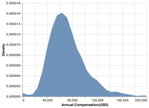
Fig. 1 Density plot of annual compensation(USD): The distribution of annual compensation is right skewed with extremely large value as well as extremely small value.¶

Among all the features investigated, it can be found that the salary is strongly correlated to the number of professional coding years. Fig.2 clearly shows that there is a linear relationship between the number of professional coding years and the salary. Figure.3 displays both effects of professional coding years and languages mastered on the salary.

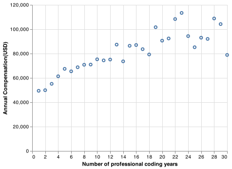
Fig. 2 Coding year vs. annual compensation(USD): Number of coding years is strongly correlated to compensation, but becomes widely spread when the coding years are greater than 20.¶

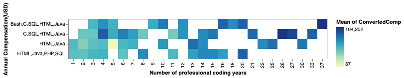
Fig. 3 Both effects of languages mastered and coding years on annual compensation: The more languages mastered and the more years in professional experience, the higher compensation expected.¶

Figures below present how other 3 features we selected have significant effects on the income level.

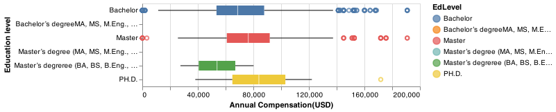
Fig. 4 Education level vs. annual compensation(USD): Education levels are positively related to compensation.¶

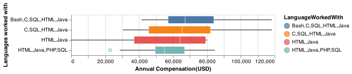
Fig. 5 Programming languages vs. annual compensation(USD): Programming languages is associated with compensation. The more programming languages mastered, the higher compensation.¶

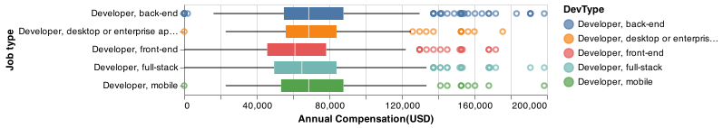
Fig. 6 Roles vs. annual compensation(USD): Roles are related to compensation. Mobile and back-end developers have greater compensation.¶

Model¶

In light of EDA and recommendations from Stack Overflow, 4 features are extracted that are duration for being a profession, education level, programming language worked with and job position. Then, the regression equation can be obtained:

\[ y_{salary} = w^T X + b \]

where w is the weight vector, X is the feature vector, b is the error term, \(y_{salary}\) is predicted variable.

Ridge model is chosen in this case, which can help reduce over-fitting problems. Ridge solves a regression model where the loss function is the linear least squares function and regularization is given by the L2-norm.

\[ loss\ function = ||y - w^T X||^2_2 + alpha * ||w||^2_2 \]

where alpha is regularization strength to reduces the variance of the estimates. Larger values specify stronger regularization.

Within the training data set, randomized hyperparameter searching was carried out based on the scoring matrix, \(R^2\). Then, the model with the best performed parameter was used to make prediction on the test data set.

Results and Discussion¶

from joblib import dump, load
import pandas as pd
from myst_nb import glue
import altair as alt
from altair_saver import save
alt.data_transformers.enable('data_server')
alt.renderers.enable('mimetype')

# Load regression training results
pipe_loaded = load('../results/best_model_pipe.joblib')
alpha = round(pipe_loaded.best_params_['ridge__alpha'], 3)
rsquare = round(pipe_loaded.best_score_, 3)
glue("alpha_coef", alpha);
glue("R2", rsquare);

# Load regression testing results
test_result_loaded = load('../results/test_result.joblib')
rsquare_test = round(test_result_loaded["r_sq_test"], 3)
glue("R2_test", rsquare_test);

# Draw the predicted value error plot
test_df = pd.read_csv("../data/processed/test.csv")
y_test = test_df.ConvertedComp.tolist()
y_predict = test_result_loaded["predict_y"].tolist()
result = {"true_y": y_test, "predicted_y": y_predict}
df_result = pd.DataFrame(data=result)
df_result.head(5)

df_diag = pd.DataFrame(data={"true_y": [0, max(df_result.true_y)+500],
                             "predicted_y":[0, max(df_result.true_y)+500]})

plt1 = alt.Chart(df_result).mark_point(opacity=0.5).encode(
    alt.X("predicted_y", title="Predicted salary"),
    alt.Y("true_y", title="True salary")
) + alt.Chart(df_diag).mark_line(color='red').encode(
    alt.X("predicted_y", title="Predicted salary"),
    alt.Y("true_y", title="True salary")
)
plt1.save("../results/test_data_result.png")

0.091

0.725

0.718

As mentioned previously, Ridge model is selected in order to avoid conditioning problems and large estimator coefficients. Firstly, hypeparameterization of alpha is carried out. The hyperparameter tuning result shows that the model is at the best performance when alpha = 0.091 with a training \(R^2\) of 0.725 as shown in the figure below.

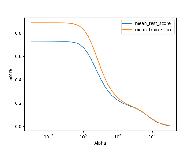
Fig. 7 Hyperparameter searching: the model is well trained when the hyperparameter, alpha, equals to 0.091. With a greater alpha, the model is under-fitted, whereas the model is over-fitted if alpha is getting smaller than 0.091.¶

Applying the fitted model to the test data set, we get a testing \(R^2\) of 0.718.

After identifying the most important features, we built multiple linear regression models with the annual salary as our response variable and the following predictors: years of coding experience, programming languages used, education level, and role. Since our target is a continuous variable, regression made sense here.

We carried out hyper-parameter tuning via cross validation with RandomizedSearchCV. This allowed us to find optimal parameters which improved our validation score from 67% to 72%. We tested the final model on our test data (20% of the survey data) and the model performed well on the test data with an accuracy of 71%. As you can see in Fig 8, the model is slightly under predicting or over-predicting, but the fit seems to be good. This is a decent score that indicates that our model generalizes enough and should perform well on unseen examples.

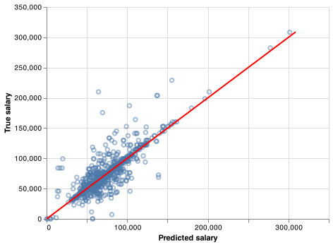
Fig. 8 Predicted salary VS. observed salary: the fitted model can fairly predict the salary.¶

Conclusions¶

In brief, our linear regression model uses 4 features (that are years of coding experience, programming languages used, education level, and role) to predict salary. It predicts with a \(R^2\) score of 0.718 on the test data set, which performs fairly well. Meanwhile, our work has shown that the salary is closely related to these 4 features.

However, there are still limitations in our work. We just used a small part of data from the survey and we are inclined to explore more features to boost the robustness and accuracy of our prediction results. Hence, in the future, we plan to do two important changes; exploring other explanatory variables that might give us a better score, and including the United States in our model. In order to identify the best features that contribute to the prediction, we will include all the sensible columns in the original survey, and perform model and feature selection. We hope that this will help us discover more features that are important for the annual compensation prediction of tech employees.

Reference¶

Sil21: Julia Silge. 2021 developer survey. 2021. URL: https://insights.stackoverflow.com/survey/2021 (visited on 2021-11-27).
VGH+18: Jacob VanderPlas, Brian Granger, Jeffrey Heer, Dominik Moritz, Kanit Wongsuphasawat, Arvind Satyanarayan, Eitan Lees, Ilia Timofeev, Ben Welsh, and Scott Sievert. Altair: interactive statistical visualizations for python. Journal of open source software, 3(32):1057, 2018.
Com20: Executable Books Community. Jupyter Book. February 2020. URL: https://doi.org/10.5281/zenodo.4539666, doi:10.5281/zenodo.4539666.
PVG+11: F. Pedregosa, G. Varoquaux, A. Gramfort, V. Michel, B. Thirion, O. Grisel, M. Blondel, P. Prettenhofer, R. Weiss, V. Dubourg, J. Vanderplas, A. Passos, D. Cournapeau, M. Brucher, M. Perrot, and E. Duchesnay. Scikit-learn: machine learning in Python. Journal of Machine Learning Research, 12:2825–2830, 2011.

Milestone Project