Predicting Wine Quality from Physicochemical Features
Authors: Gabriel Fairbrother, Paniz Fazlali, Luming Yang, Wanying Ye; The University of British Columbia, Master of Data Science.
2021-12-11
Summary
This project is an attempt to build a classification model for predicting wine quality. We have two main questions. First, can we use a machine learning model to predict the human perceived quality of a wine using its physical and chemical attributes? Second, which of these attributes contribute most to that perceived quality?
We evaluated three models including Logistic Regression, Support Vector Machine with linear kernel (SVC linear) and Random Forest Classification. Our best classifier was Random Forest Classifier, with the best validation ROC AUC (One vs Rest) score of 0.867 through hyperparameter optimization. The test ROC AUC (One vs Rest) score for Random Forest Classifier was 0.685. The confusion matrix implies that the model did a fairly good job - most of the false predictions fall into adjacent classes, which makes sense because our target classes are indeed ordinal. The feature importances given by this optimized model suggested that alcohol, density and volatile acidity are the top 3 contributing features in this prediction task. In general, we are confident to use and share this model as a preliminary tool to classify the quality scores of red and white wines. We recommend further improvement on feature engineering to extract better features and increase the model performance.
Introduction
Wine is both an extremely popular and highly consumed product, one that can be very expensive to buy and lucrative to sell. It is also sold at much higher variety levels than almost any other consumer product - in some supermarkets well over 1000 different wines are stocked.[Lockshin, 2003]
At the same time, it is also one of the hardest to identify quality ahead of purchase, since you must consume it to decide. The level of quality a consumer might require can even vary wildly depending on the consumption occasion [Quester and others, 1998]
The quality of wine is difficult to evaluate objectively and is reliant on some very subjective sensory elements. However we believe that this question can be answered by evaluating which physicochemical features are important in determining the quality score of a wine. We also believe that by using a quality score that is a human taste output (i.e. each quality score is a median taken over a minimum of 3 sensory assessors) instead of following an objective and rigid standard (which makes wine certification a complicated task), we can better capture the inherent subjectivity of the task. Therefore, attempting to unravel the relationship between physicochemical properties and human taste sensations may also be a direction in the wine certification field [Cortez, Cerdeira, Almeida, Matos, and Reis, 2009]
We believe that using a machine learning model to predict the human perceived quality can be useful in multiple wine-related industries to help retailers choose more desirable wine selections for consumers and also help producers focus their processes to create higher quality wines.
Methods
Data
The data sets used in this project were sampled from the red and white vinho verde wines from the North of Portugal, created by Paulo Cortez, António Cerdeira, Fernando Almeida, Telmo Matos, and José Reis [Cortez et al., 2009]. They were sourced from the UC Irvine Machine Learning Repository [Dua and Graff, 2017] and can be found here. One data set is for the red wine, and the other is for the white wine, and both data sets have the same features and target columns. We combined these columns and created a new feature to indicate colour. Each row represents a wine sample with its physicochemical properties such as fixed acidity, volatile acidity, etc. The target is a score (integer but we treat as a classification task) ranging from 3 (very bad) to 9 (excellent) that represents the quality of the wine.
Here is a breakdown of the number of examples in the train and test set:
Train Set Size |
Test Set Size |
|---|---|
4547 |
1950 |
Analysis
Three classification models were attempted and assessed to predict the quality score of a wine: Logistic Regression, Support Vector Machine with linear kernel (SVC linear) and Random Forest Classification. These candidates were selected based on their common intriguing attributes such as high interpretability and giving handy measurements on feature importance. All numeric features in the original datasets were included and scaled, with the type of wine (i.e. white or red) as an added binary feature.
During the EDA stage, we discovered the data set has severe class-imbalance issue as shown in (Fig. 1). Our target is multi-class in terms of quality scores ranging from “3” to “9”. However, the classes “3” and “9” were extremely under-populated. Therefore, we decided to combine the lowest two classes (“3” and “4”) and the highest two classes (“8” and “9”) to mitigate the severe class imbalance problem. By doing so, the number of examples in each class is distributed more evenly. The final quality score classes are “<=4”, “5”, “6”, “7” and “>=8”. The best wines will be classified as “>=8”, and the poorest wines will be classified as “<=4”.
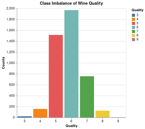
Fig. 1 Class imbalance in original data.
We also chose the scoring metrics to be f-1 macro score, Receiver Operating Characteristic (One vs. Rest) Area Under the Curve, and Receiver Operating Characteristic (One vs. One) Area Under the Curve.
For each algorithm, the default hyperparameters were used first to train the model, and then the 5-fold cross-validation scores were compared across the models. Hyperparameter optimization was carried out on the algorithm with the best cross-validation score. The resulting model with the optimized hyperparameters was the solution to this prediction task. We then assess its performance on test data (i.e. unseen examples).
The computing language used in this project is Python [Perez et al., 2011]. Packages used in EDA and machine learning analysis include: altair [VanderPlas et al., 2018], docopt [de Jonge, 2020], scikit-learn [Pedregosa et al., 2011], matplotlib [Hunter, 2007], numpy [Harris et al., 2020], pandas [McKinney and others, 2010], pickle [Van Rossum, 2020].
Results & Discussion
To see whether there is some relation between different features and also to have an idea on whether some features are more important in prediction, we explored the correlation plot for all numeric features and the wine quality score. As shown in Fig. 2, several features have strong correlation. For example, total sulfur dioxide and free sulfur dioxide are strongly positively correlated, and alcohol and density are strongly negatively correlated. Additionally, the high correlation between the target quality and some features (i.e. alcohol, density, chlorides, volatile acidity) imply that these features might be important for prediction.

Fig. 2 Correlation plot for all numeric features (excluding wine type) and quality score.
In order to classify the wine qualities, we chose to use three different models, including support vector machine with linear kernel, logistic regression, and random forest. We carried out 5-fold cross validation on all three models to find the best performing model based on the cross validation scores. During the EDA stage of the project, we observed class imbalance in our data set. Therefore, we decided to use several scoring metrics such as f1 score, Receiver Operating Characteristic - One versus Rest - Area under the curve (ROC-AUC-OVR), and Receiver Operating Characteristic - One versus One - Area under the curve (ROC-AUC-OVO).
Based on the cross validation results shown in Table. 1, the random forest model performed the best across three models. Therefore, the random forest model was selected for downstream hyperparamater tuning.
Table. 1 Summary on f1 macro scores, ROC AUC (OVR) and ROC AUC (OVO) of dummy classifier, SVC, logistic regression, and random forest with default hyperparameters.
import pandas as pd
pd.read_csv("../../results/cross_val_results.csv", index_col = 0)
| fit_time | score_time | test_accuracy | train_accuracy | test_f1_macro | train_f1_macro | test_roc_auc_ovr | train_roc_auc_ovr | test_roc_auc_ovo | train_roc_auc_ovo | |
|---|---|---|---|---|---|---|---|---|---|---|
| Dummy | 0.009 (+/- 0.002) | 0.021 (+/- 0.001) | 0.333 (+/- 0.013) | 0.333 (+/- 0.004) | 0.193 (+/- 0.011) | 0.200 (+/- 0.005) | 0.496 (+/- 0.007) | 0.501 (+/- 0.003) | 0.496 (+/- 0.007) | 0.500 (+/- 0.003) |
| SVC | 3.100 (+/- 0.110) | 0.185 (+/- 0.011) | 0.532 (+/- 0.017) | 0.539 (+/- 0.004) | 0.241 (+/- 0.008) | 0.244 (+/- 0.002) | 0.746 (+/- 0.011) | 0.755 (+/- 0.009) | 0.730 (+/- 0.012) | 0.738 (+/- 0.010) |
| Logistic Regression | 0.199 (+/- 0.013) | 0.024 (+/- 0.002) | 0.546 (+/- 0.014) | 0.550 (+/- 0.004) | 0.325 (+/- 0.012) | 0.330 (+/- 0.005) | 0.764 (+/- 0.016) | 0.777 (+/- 0.003) | 0.759 (+/- 0.014) | 0.772 (+/- 0.003) |
| Random Forest | 0.593 (+/- 0.042) | 0.070 (+/- 0.001) | 0.652 (+/- 0.012) | 1.000 (+/- 0.000) | 0.501 (+/- 0.025) | 1.000 (+/- 0.000) | 0.852 (+/- 0.003) | 1.000 (+/- 0.000) | 0.847 (+/- 0.003) | 1.000 (+/- 0.000) |
To find the best parameters of the random forest model, we perform hyperparameter optimization on n_estimators and max_depth in the random forest model. The optimal hyperparameter results are shown in the Table. 2. We observed that the optimal n_estimators was 4641 and the max_depth was 26. During the hyperparameter optimization, we used roc_auc_ovr as our scoring metrics. The validation score for the optimized model is 0.867, and the test score for the optimized model is 0.685.
Table. 2 The best ROC-AUC-OVR cross-validation score together with the hyperparameter combination yielding the it, and the test score of this tuned random forest model on test examples.
pd.read_csv("../../results/random_forest_results.csv", index_col = 0).round(3)
| Random Forest Best n_estimators | Random Forest Best max_depth | Random Forest Best Validation Score | Random Forest Roc_Auc Test Score | |
|---|---|---|---|---|
| 0 | 4641 | 26 | 0.867 | 0.685 |
In addition, we plotted the confusion matrix of model performance on test data to get insights of how our model performed. As seen in Fig. 3, our model was mostly confused among the quality classes of “5”, “6” and “7”. This is probably because the features do not have well separated distributions with respect to these classes. This is in line with what we observed in the preliminary exploratory data analysis. Although the model did not perform great on this classification task, our main task does not include any sensitive prediction. Therefore, we are relatively confident to share the results of our model.
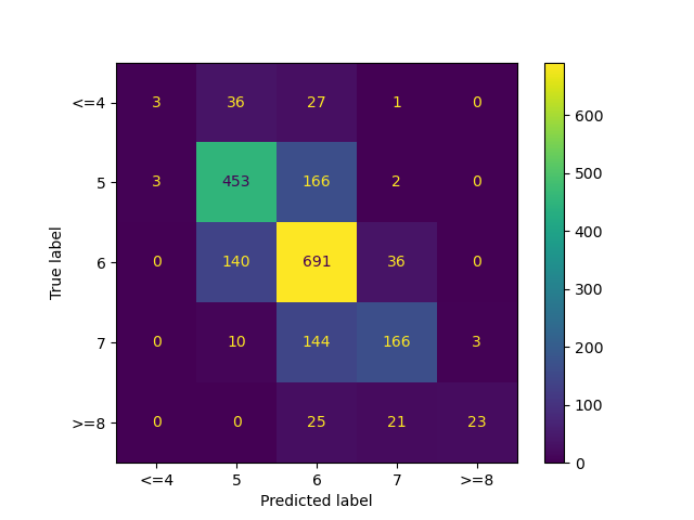
Fig. 3 Confusion matrix on test data.
Among all the features that our data set had, alcohol, density and volatile acidity were the top 3 important features (see Table. 3). On the other hand, fixed acidity, type_white and type_red were the least important features. This result is also consistent with our initial exploratory data analysis.
Table. 3 The feature importances of the optimized random forest model.
pd.read_csv("../../results/feature_importances.csv", index_col = 0).round(3)
| Feature Importances | |
|---|---|
| alcohol | 0.116 |
| density | 0.094 |
| volatile acidity | 0.091 |
| total sulfur dioxide | 0.082 |
| chlorides | 0.079 |
| free sulfur dioxide | 0.079 |
| residual sugar | 0.077 |
| sulphates | 0.076 |
| pH | 0.073 |
| citric acid | 0.071 |
| fixed acidity | 0.067 |
| type_white | 0.003 |
| type_red | 0.003 |
Conclusions
In conclusion, the random forest model seems to be a good candidate for this quality prediction task, and the tuned random forest model ranks alcohol, density and volatile acidity as the 3 most important features. However, due to the presence of a almost 20% gap between the cross-validation score and the test score, whether this model will generalize well to real-world unseen data remains a doubt.
Limitations & Future Work
Firstly, we suggest gathering more wine samples from lower quality class and higher quality class to fix the severe class imbalance issue in the dataset so that it could be used to classify the wine qualities properly in the real world. Additionally, to improve the model performance in future, we could carry out feature engineering such as adding polynomial features or creating new features under domain expertise, and perform feature elimination to remove unimportant features. It may also be worth diversifying the wine types to other regions and varietals.
Bibliography
- CCA+09
Paulo Cortez, António Cerdeira, Fernando Almeida, Telmo Matos, and José Reis. Modeling wine preferences by data mining from physicochemical properties. Decision support systems, 47(4):547–553, 2009.
- DG17
Dheeru Dua and Casey Graff. UCI machine learning repository. 2017. URL: http://archive.ics.uci.edu/ml.
- HMvdW+20
Charles R. Harris, K. Jarrod Millman, Stéfan J. van der Walt, Ralf Gommers, Pauli Virtanen, David Cournapeau, Eric Wieser, Julian Taylor, Sebastian Berg, Nathaniel J. Smith, Robert Kern, Matti Picus, Stephan Hoyer, Marten H. van Kerkwijk, Matthew Brett, Allan Haldane, Jaime Fernández del Río, Mark Wiebe, Pearu Peterson, Pierre Gérard-Marchant, Kevin Sheppard, Tyler Reddy, Warren Weckesser, Hameer Abbasi, Christoph Gohlke, and Travis E. Oliphant. Array programming with NumPy. Nature, 585(7825):357–362, September 2020. URL: https://doi.org/10.1038/s41586-020-2649-2, doi:10.1038/s41586-020-2649-2.
- Hun07
J. D. Hunter. Matplotlib: a 2d graphics environment. Computing in Science & Engineering, 9(3):90–95, 2007. doi:10.1109/MCSE.2007.55.
- Loc03
Larry Lockshin. Consumer purchasing behaviour for wine: what we know and where we are going. Academia.edu, 2003. URL: https://www.academia.edu/32936140/Consumer_Purchasing_Behaviour_for_Wine_What_We_Know_and_Where_We_are_Going.
- M+10
Wes McKinney and others. Data structures for statistical computing in python. In Proceedings of the 9th Python in Science Conference, volume 445, 51–56. Austin, TX, 2010.
- PVG+11
F. Pedregosa, G. Varoquaux, A. Gramfort, V. Michel, B. Thirion, O. Grisel, M. Blondel, P. Prettenhofer, R. Weiss, V. Dubourg, J. Vanderplas, A. Passos, D. Cournapeau, M. Brucher, M. Perrot, and E. Duchesnay. Scikit-learn: machine learning in Python. Journal of Machine Learning Research, 12:2825–2830, 2011.
- PGH11
Fernando Perez, Brian E Granger, and John D Hunter. Python: an ecosystem for scientific computing. Computing in Science \\& Engineering, 13(2):13–21, 2011.
- Q+98
P. G. Quester and others. The influence of consumption situation and product involvement over consumers' use of product attribute. Journal of Consumer Marketing, 1998. URL: https://doi.org/10.1108/07363769810219107.
- VR20
Guido Van Rossum. The Python Library Reference, release 3.8.2. Python Software Foundation, 2020.
- VGH+18
Jacob VanderPlas, Brian Granger, Jeffrey Heer, Dominik Moritz, Kanit Wongsuphasawat, Arvind Satyanarayan, Eitan Lees, Ilia Timofeev, Ben Welsh, and Scott Sievert. Altair: interactive statistical visualizations for python. Journal of open source software, 3(32):1057, 2018.
- deJonge20
Edwin de Jonge. docopt: Command-Line Interface Specification Language. 2020. R package version 0.7.1. URL: https://CRAN.R-project.org/package=docopt.