RidgeMake Tutorial
RidgeMake Workflow Tutorial
This guide provides a functional overview of a four-step workflow for performing linear regression, evaluating model performance, and visualizing results using NumPy and Matplotlib.
| Function | Purpose | Key Mechanism |
|---|---|---|
| get_reg_line | Fit & Predict | Uses the Normal Equation to calculate optimal weights and return predictions. |
| ridge_get_r2 | Evaluate | Computes the R2 score to measure the proportion of variance captured by the model. |
| ridge_scatter | Visualize (Data) | Plots the raw observations (x,y) onto a Matplotlib Axes object. |
| ridge_scatter_line | Visualize (Model) | Overlays the predicted regression line onto the existing scatter plot. |
Implementataion Example
import numpy as np
import matplotlib.pyplot as plt
from ridge_remake.get_reg_line import get_reg_line
from ridge_remake.ridge_r2 import ridge_get_r2
from ridge_scatter_line import ridge_scatter_line
from ridge_scatter import ridge_scatter
# 1. Generate Synthetic Data
np.random.seed(42)
X = 2 * np.random.rand(50, 1)
y = 4 + 3 * X + np.random.randn(50, 1) # y = 4 + 3x + noise# 2. Compute Predictions
# get_reg_line handles the bias term internally via the Normal Equation
y_pred = get_reg_line(X, y)# 3. Calculate Model Accuracy
r2_score = ridge_get_r2(y, y_pred)
print(f"Model R² Score: {r2_score:.4f}")Model R² Score: 0.7683
# 4. Visualization
fig, ax = plt.subplots(figsize=(8, 5))

# Plot raw data
ridge_scatter(ax, X, y, label="Observed Data", scatter_kwargs={"color": "blue", "alpha": 0.6})
plt.show()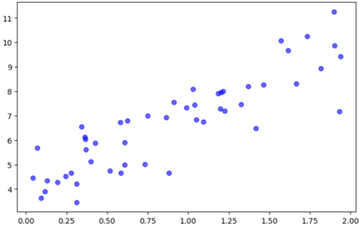
# Plot regression line
ridge_scatter_line(ax, X, y_pred, label=f"Regression Line (R²={r2_score:.2f})",
                   line_kwargs={"color": "red", "linewidth": 2})

ax.set_xlabel("Independent Variable (X)")
ax.set_ylabel("Target (y)")
ax.set_title("Simple Linear Regression Fit")
ax.legend()
plt.show()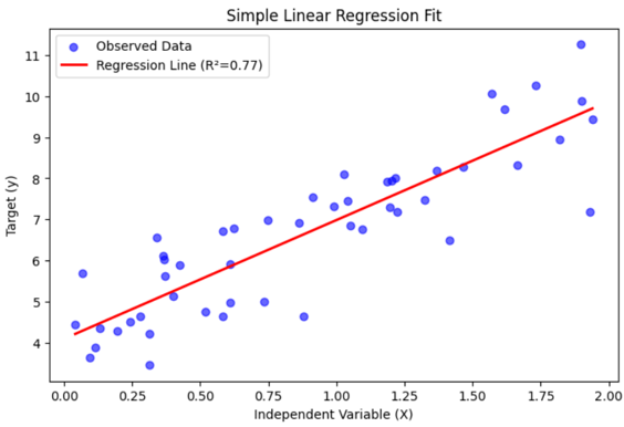
Key Technical Considerations
Matrix Operations: get_reg_line relies on np.linalg.inv. Note that for high-dimensional data or collinear features, the matrix XTX may be singular (non-invertible).
The Bias Term: The prediction function automatically prepends a column of ones to the input matrix. This ensures the model accounts for the intercept (β0), preventing the line from being forced through the origin.
Sorting for Plots: ridge_scatter_line includes a sort_x=True parameter. This is critical when working with shuffled data; without it, Matplotlib connects points in their index order, resulting in a “zig-zag” mess rather than a clean line.
R2 Interpretation:
1.0: Perfect fit.
0.0: Model predicts no better than the mean of y.
Negative: The model is worse than simply predicting the mean (usually indicates a non-linear trend or severe overfit on training data).