RPrelimEdaHelper-vignette

Setting up the library

library(RPrelimEdaHelper)

Lets look at some examples using PalmerPenguins Package

library (palmerpenguins)

penguins<- tidyr::drop_na(penguins)
head(penguins)
#> # A tibble: 6 × 8
#>   species island    bill_length_mm bill_depth_mm flipper_l…¹ body_…² sex    year
#>   <fct>   <fct>              <dbl>         <dbl>       <int>   <int> <fct> <int>
#> 1 Adelie  Torgersen           39.1          18.7         181    3750 male   2007
#> 2 Adelie  Torgersen           39.5          17.4         186    3800 fema…  2007
#> 3 Adelie  Torgersen           40.3          18           195    3250 fema…  2007
#> 4 Adelie  Torgersen           36.7          19.3         193    3450 fema…  2007
#> 5 Adelie  Torgersen           39.3          20.6         190    3650 male   2007
#> 6 Adelie  Torgersen           38.9          17.8         181    3625 fema…  2007
#> # … with abbreviated variable names ¹​flipper_length_mm, ²​body_mass_g

Here are some examples of how the functions work

num_dist_by_cat(
  num = bill_depth_mm, group = sex, data = penguins,
  title_hist = 'Distribution of bill length', title_boxplot = 'Bill length by group',
  lab_num = 'Bill length (mm)', lab_group = 'Sex' ,  num_on_x = TRUE, stat = TRUE)
#>                    Test         t            p
#> 1    Equal var. assumed -7.306540 2.066410e-12
#> 2 Equal var. not asumed -7.308982 2.035676e-12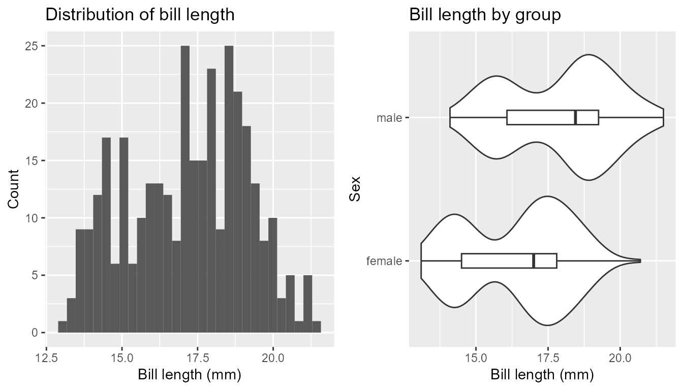

num_dist_summary(
  col_name ="bill_depth_mm", data= tidyr::drop_na(penguins), title='Bill Depth (mm) ',label_x= 'distribution of Bill Depth ', 
  thresh_corr = 0.3,stat = TRUE
)
#> [1] "Summary statistics \n"
#> # A tibble: 1 × 5
#>   column        num_na  mean median stdev
#>   <chr>          <int> <dbl>  <dbl> <dbl>
#> 1 bill_depth_mm      0  17.2   17.2  1.97
#> [1] "Correlation Values \n"
#> # A tibble: 1 × 2
#>   features      correlation
#>   <chr>               <dbl>
#> 1 bill_depth_mm           1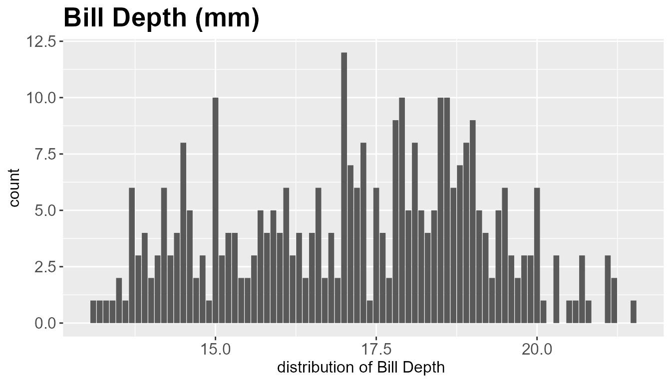

num_dist_scatter(num1='bill_length_mm', num2='body_mass_g', data=penguins,
                      title = 'num1 vs num2', stat=TRUE, trend= 'loess')
#> # A tibble: 2 × 5
#>   column         num_na   mean median  stdev
#>   <chr>           <int>  <dbl>  <dbl>  <dbl>
#> 1 bill_length_mm      0   44.0   44.0   5.47
#> 2 body_mass_g         0 4207.  4207.  805.  
#> 
#>  iter imp variable
#>   1   1
#> Warning in cor.test.default(df1[[num1]], df1[[num2]], method = "spearman", :
#> Cannot compute exact p-value with ties

#> Warning in cor.test.default(df1[[num1]], df1[[num2]], method = "spearman", :
#> Cannot compute exact p-value with ties
#> # A tibble: 2 × 3
#>   Method     Correlation  P_value
#>   <chr>            <dbl>    <dbl>
#> 1 Pearson's        0.589 1.54e-32
#> 2 Spearman's       0.576 6.97e-31
#> `geom_smooth()` using formula = 'y ~ x'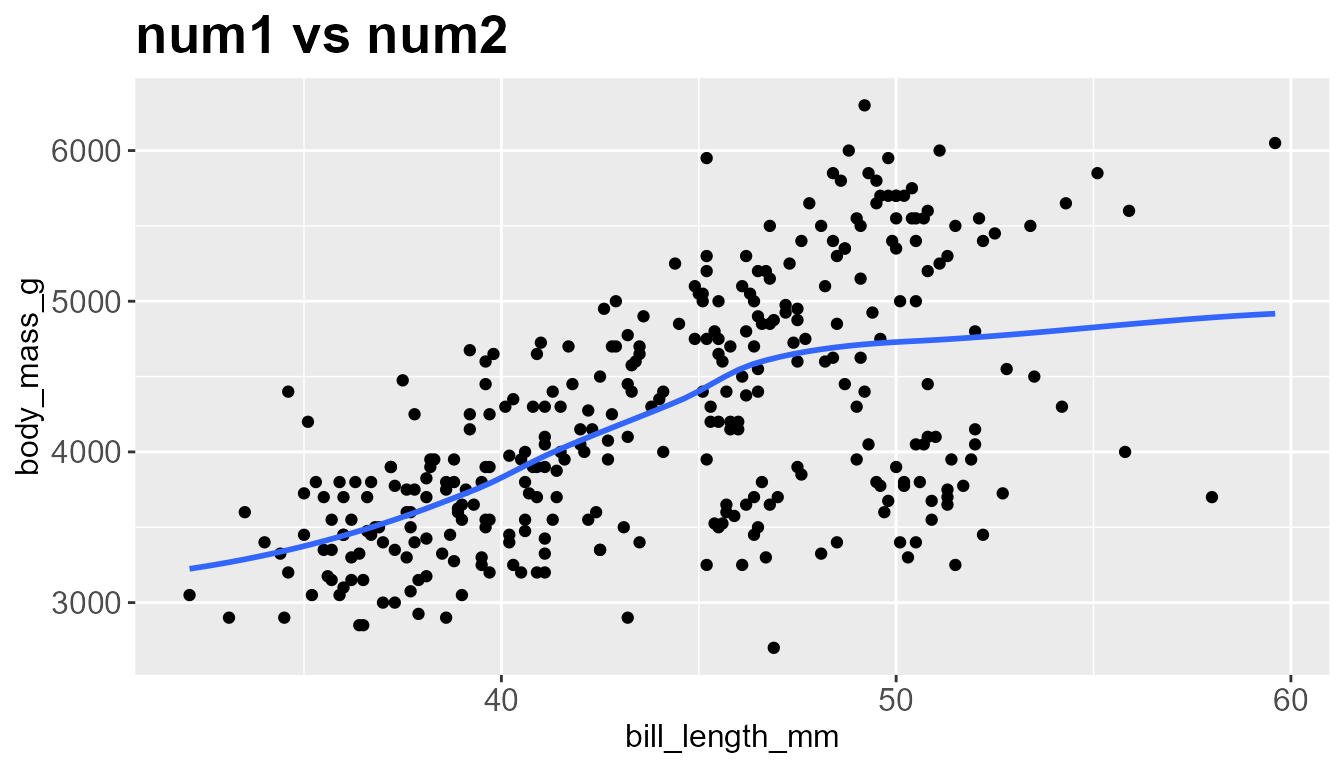

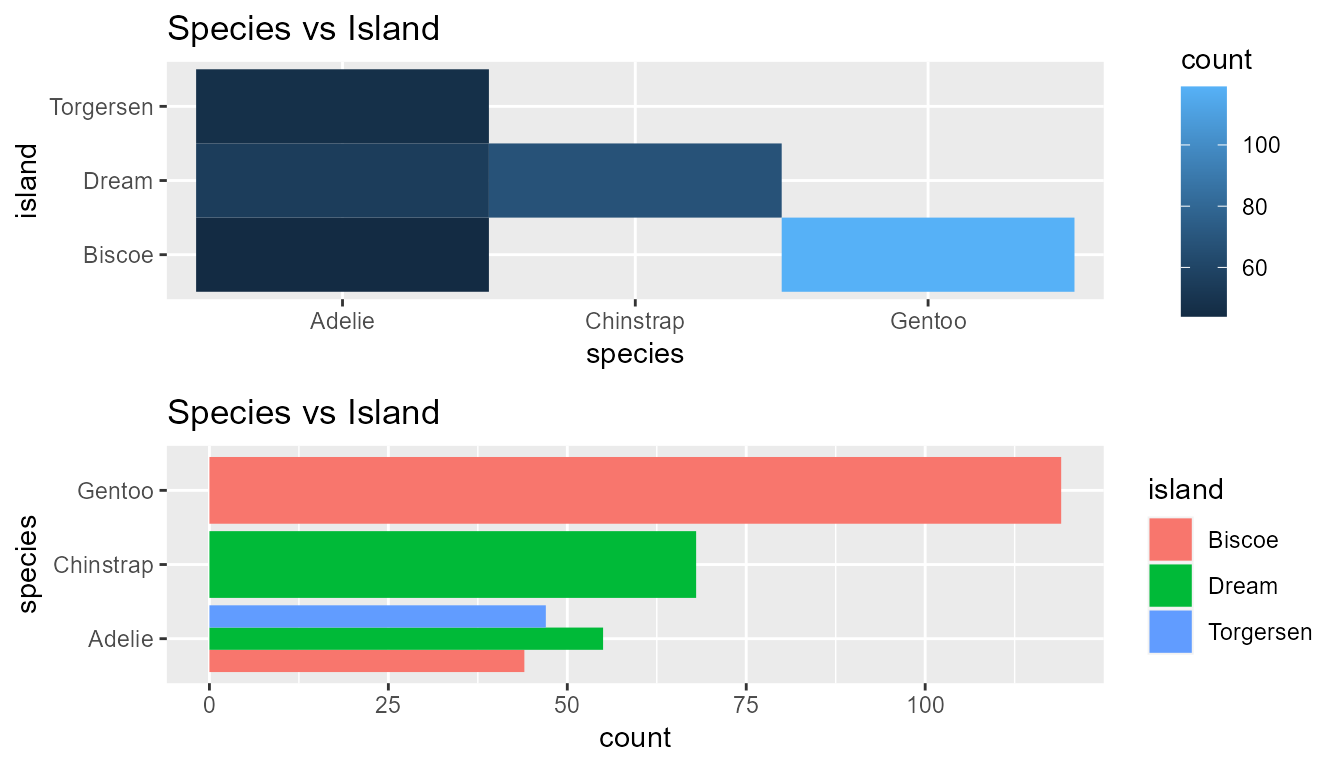
cat_dist_heatmap(cat_1 = 'species', cat_2 = 'island', data = penguins, title = 'Species vs Island',
                 heatmap = TRUE, barchart = TRUE)
#> Warning: Use of `data[[cat_1]]` is discouraged.
#> ℹ Use `.data[[cat_1]]` instead.
#> Warning: Use of `data[[cat_2]]` is discouraged.
#> ℹ Use `.data[[cat_2]]` instead.
#> Warning: Use of `data[[cat_1]]` is discouraged.
#> ℹ Use `.data[[cat_1]]` instead.
#> Warning: Use of `data[[cat_2]]` is discouraged.
#> ℹ Use `.data[[cat_2]]` instead.