hueniverrrsity-vignette

library(hueniverrrsity)
library(ggplot2)

Introduction

All universities and colleges have a visual identity composed of their specific colours and typefaces. This enables all publications from a given university to have a cohesive theme and be immediately identifiable.

hueniverrrsity is a package designed to apply the visual themes of four Canadian Universities to ggplot2 objects. The package currently supports the visual identities of University of Alberta, McGill University, the University of Toronto, and the University of British Columbia.

Functions

• theme_alberta() - Applies the U of A visual identity to ggplot2 objects. Input:

  • colour_use: fill or colour
    • colour_use = colour for geom_point() and geom_line()
    • colour_use = fill for geom_boxplot(), geom_bar(), geom_violin() and geom_histogram()
  • colour_palette: alpha, beta, gamma or delta colour palettes are different colour combinations specified in the U of A visual identity

• theme_mcgill() - Applies the McGill visual identity to ggplot2 objects.

  Input:

  • colour_use: fill or colour
    • colour_use = colour for geom_point() and geom_line()
    • colour_use = fill for geom_boxplot(), geom_bar(), geom_violin() and geom_histogram()

• theme_toronto() - Applies the U of T visual identity to ggplot2 objects.

  Input:

  • colour_use: fill or colour
    • colour_use = colour for geom_point() and geom_line()
    • colour_use = fill for geom_boxplot(), geom_bar(), geom_violin() and geom_histogram()
  • colour_palette: vibrant, cool or awards colour palettes are different colour combinations specified in the U of T visual identity

• theme_ubc() - Applies the UBC visual identity to ggplot2 objects.

  Input:

  • colour_use: fill or colour
    • colour_use = colour for geom_point() and geom_line()
    • colour_use = fill for geom_boxplot(), geom_bar(), geom_violin() and geom_histogram()

Examples

• theme_alberta()

# Create scatter plot
ggplot(data=mtcars, aes(x = hp, y = mpg, colour = as.factor(cyl))) +
  geom_point(size = 3, alpha = 0.8) +
  theme_alberta('colour', 'beta')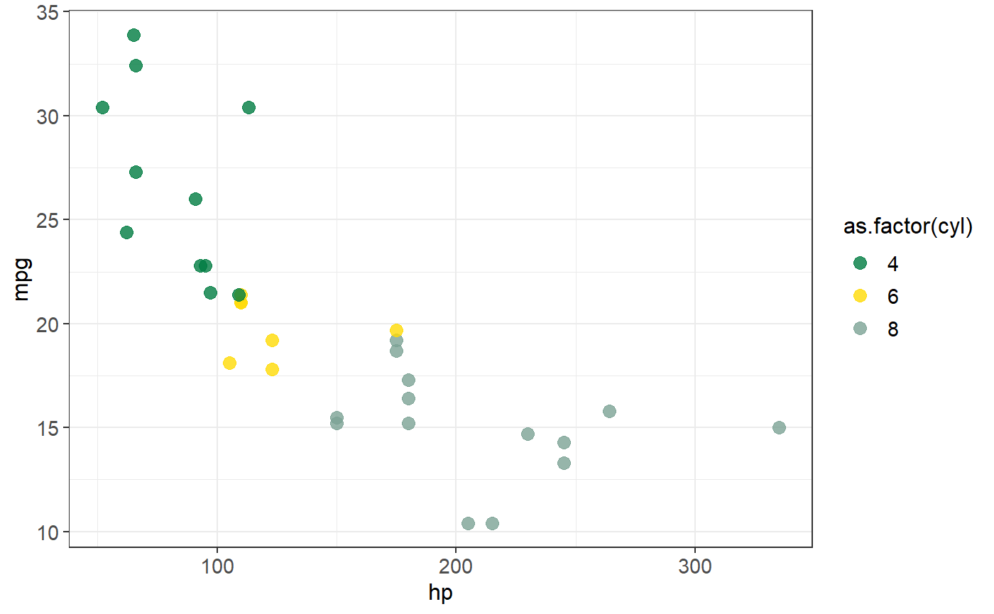

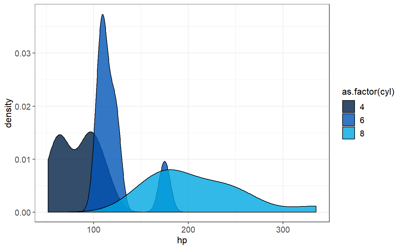
# Create density plot
ggplot(data = mtcars, aes(x = hp, fill = as.factor(cyl))) +
  geom_density(alpha = 0.8) +
  theme_alberta('fill', 'delta')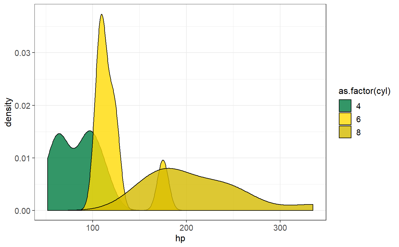

• theme_mcgill()

# Create scatter plot
ggplot(data = mtcars, aes(x = hp, y = mpg, colour = as.factor(cyl))) +
  geom_point(size = 3, alpha = 0.8) +
  theme_mcgill('colour')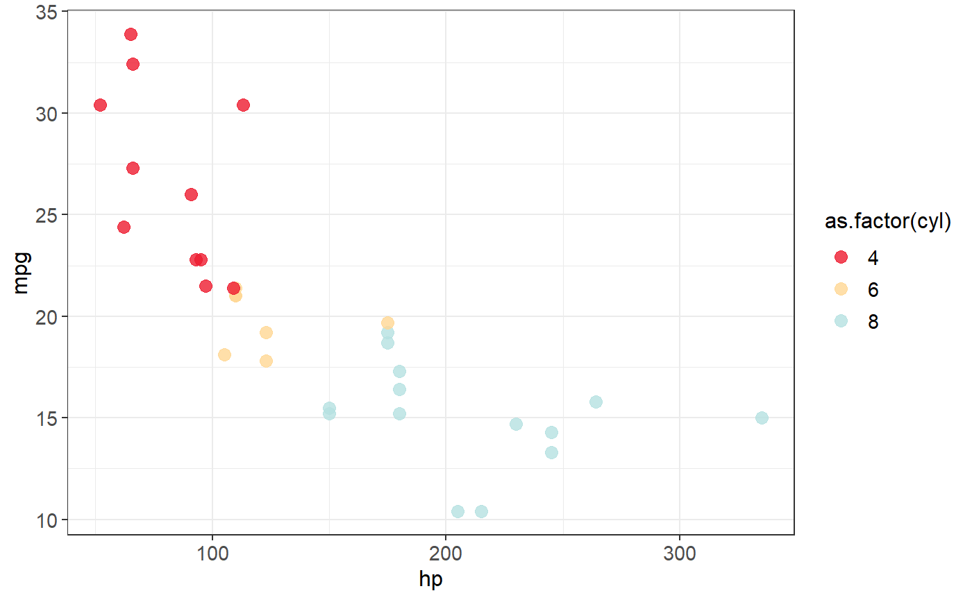

# Create density plot
ggplot(data = mtcars, aes(x = hp, fill = as.factor(cyl))) +
  geom_density(alpha=0.8) +
  theme_mcgill('fill')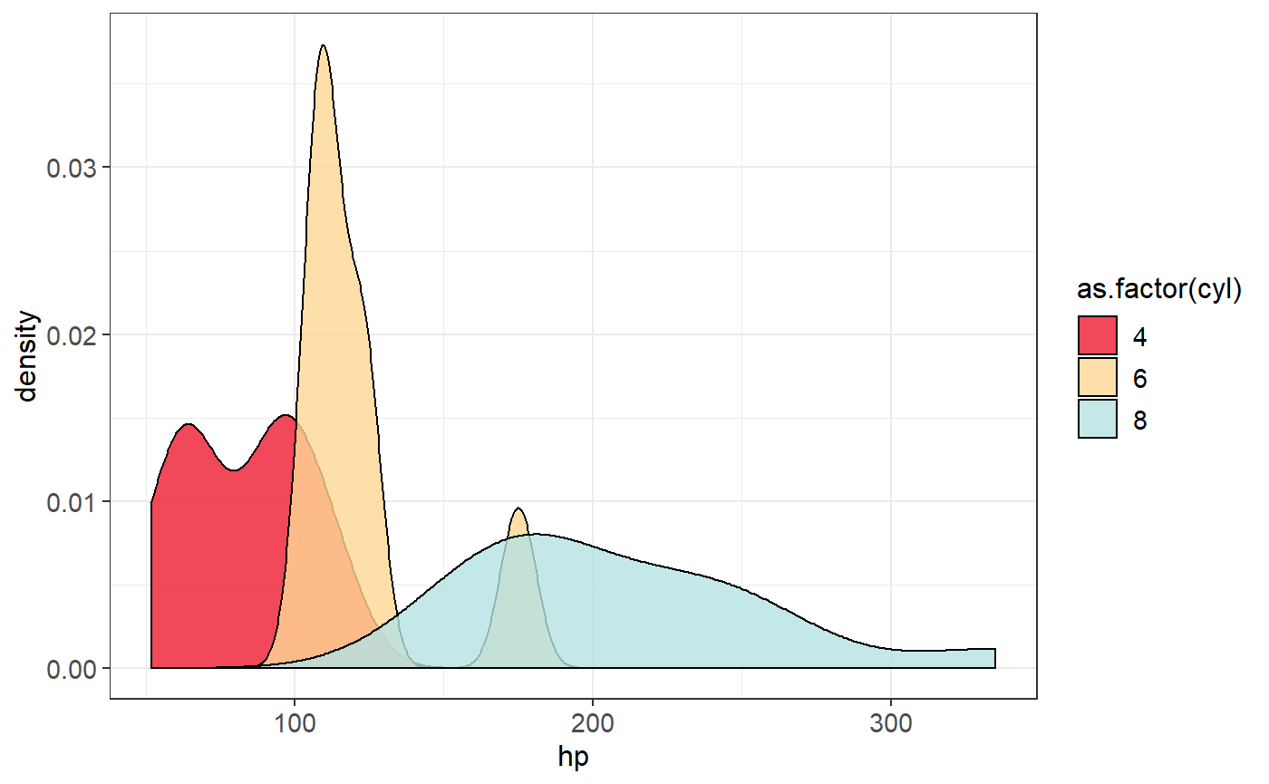

• theme_toronto()

# Create scatter plot
ggplot(data = mtcars, aes(x = hp, y = mpg, colour = as.factor(cyl))) +
  geom_point(size = 2.5) +
  theme_toronto('colour', 'vibrant')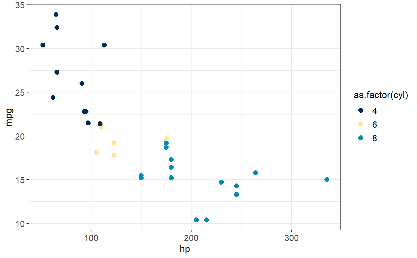

# Create density plot
ggplot(data = mtcars, aes(x = hp, fill = as.factor(cyl))) +
  geom_density(alpha = 0.8) +
  theme_toronto('fill', 'awards')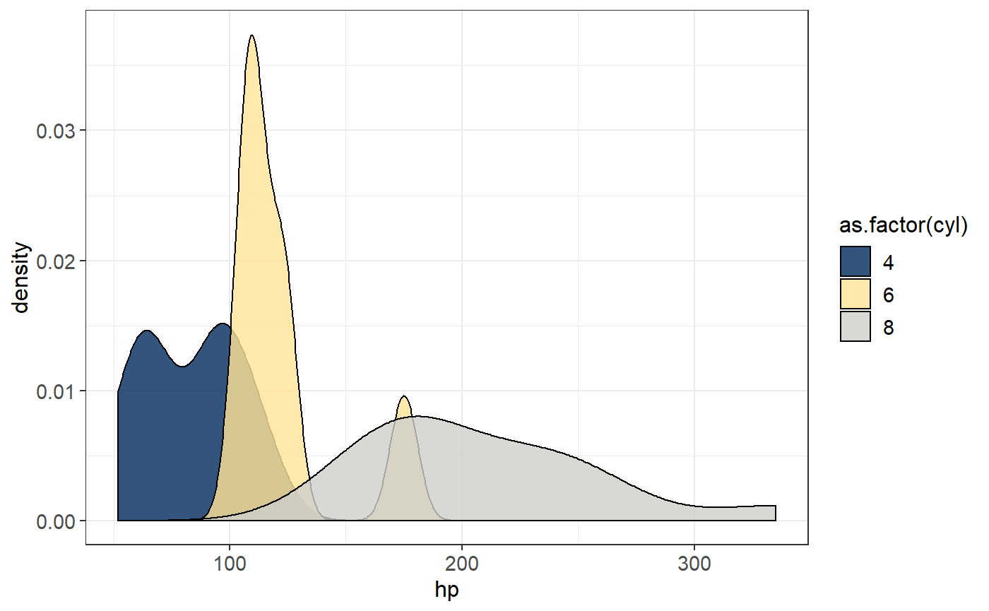

• theme_ubc()

# Create scatter plot
ggplot(data = mtcars, aes(x = hp, y = mpg, colour = as.factor(cyl))) +
  geom_point(size = 2.5) +
  theme_ubc('colour')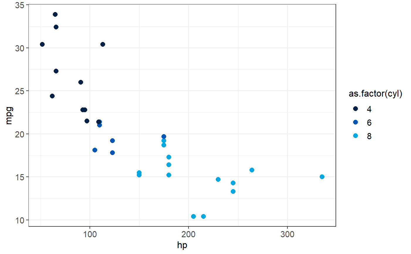

# Create density plot
ggplot(data = mtcars, aes(x = hp, fill = as.factor(cyl))) +
  geom_density(alpha=0.8) +
  theme_ubc('fill')