Introduction
The functions in nurser were developed to provide useful and informative front-end machine learning metrics that are applicable to a wide array of datasets. Currently nurser contains three functions, each of which are independent of one another. This vignette outlines how to use these functions on some real data.
eda
The eda() function return a list that contains histogram and summary statistics for a given column. Let’s see it in action!
To view a histogram of a feature:
result <- eda(mtcars)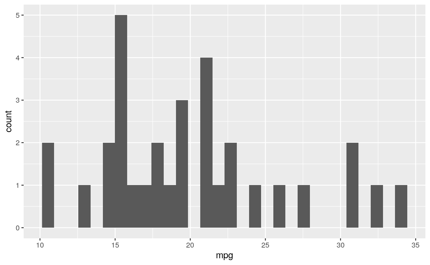
Now let’s see the summary statistics of this feature:
stats_mpg = result$stats$mpg
stats_mpg
#>    Min. 1st Qu.  Median    Mean 3rd Qu.    Max.
#>   10.40   15.43   19.20   20.09   22.80   33.90
impute_summary
Let’s import some continuous data to work with,
and add some missing values,
iris_missing <-
  as.data.frame(lapply(iris_data,
                       function(x) x[sample(c(TRUE, NA),
                                            size = length(x),
                                            replace = TRUE,
                                            prob = c(0.75, 0.25))]))
Now, let’s take a look at the data to in fact see if the missing values were generated and where they are:
iris_missing %>% head(10)
#>    Sepal.Length Sepal.Width Petal.Length Petal.Width
#> 1           5.1         3.5          1.4          NA
#> 2            NA         3.0          1.4         0.2
#> 3           4.7         3.2          1.3         0.2
#> 4           4.6         3.1           NA         0.2
#> 5           5.0         3.6          1.4         0.2
#> 6           5.4          NA          1.7          NA
#> 7           4.6         3.4          1.4         0.3
#> 8           5.0          NA          1.5         0.2
#> 9            NA         2.9          1.4         0.2
#> 10          4.9         3.1          1.5         0.1
Great, we have some missing values to compute - let’s call impute_summary to get some summary statistics and outputs from different methods.
iris_imputed <- impute_summary(iris_missing)impute_summary() provides some useful summary statistics and also several imputed dataframes that can be accessed by the impute_summary object attributes. The imputed data frames provided include:
- mean,
- median,
- max,
- min,
- random,
- multiple imputation,
- pmm, and
- random forest
Let’s first take a look at the summaries, which can be accessed using $nan_counts (NA counts for each feature) and $nan_rowindex (rows that contain NA values):
iris_imputed$nan_counts
#>              NaN_count
#> Sepal.Length        31
#> Sepal.Width         37
#> Petal.Length        40
#> Petal.Width         32
#> Total              140

iris_imputed$nan_rowindex %>% head(5)
#>   NaN_Rows
#> 1        1
#> 2        2
#> 3        4
#> 4        6
#> 5        8
Now, let’s take a look at two of the imputed data frames, mean and multiple imputation:
iris_imputed$hmisc_mean %>% head(10)
#>    Sepal.Length Sepal.Width Petal.Length Petal.Width
#> 1      5.100000    3.500000     1.400000    1.217797
#> 2      5.869748    3.000000     1.400000    0.200000
#> 3      4.700000    3.200000     1.300000    0.200000
#> 4      4.600000    3.100000     3.654545    0.200000
#> 5      5.000000    3.600000     1.400000    0.200000
#> 6      5.400000    3.065487     1.700000    1.217797
#> 7      4.600000    3.400000     1.400000    0.300000
#> 8      5.000000    3.065487     1.500000    0.200000
#> 9      5.869748    2.900000     1.400000    0.200000
#> 10     4.900000    3.100000     1.500000    0.100000

iris_imputed$mi_multimp %>% head(10)
#>    Sepal.Length Sepal.Width Petal.Length Petal.Width
#> 1      5.100000    3.500000     1.400000   0.1780005
#> 2      4.329420    3.000000     1.400000   0.2000000
#> 3      4.700000    3.200000     1.300000   0.2000000
#> 4      4.600000    3.100000     1.271374   0.2000000
#> 5      5.000000    3.600000     1.400000   0.2000000
#> 6      5.400000    3.881438     1.700000   0.2782553
#> 7      4.600000    3.400000     1.400000   0.3000000
#> 8      5.000000    3.166817     1.500000   0.2000000
#> 9      4.401506    2.900000     1.400000   0.2000000
#> 10     4.900000    3.100000     1.500000   0.1000000
preproc
The preproc() function returns a tibble with preprocessed features. Simply call preproc on your data!
Let’s first view our data before preprocessing:
head(iris)
#>   Sepal.Length Sepal.Width Petal.Length Petal.Width Species
#> 1          5.1         3.5          1.4         0.2  setosa
#> 2          4.9         3.0          1.4         0.2  setosa
#> 3          4.7         3.2          1.3         0.2  setosa
#> 4          4.6         3.1          1.5         0.2  setosa
#> 5          5.0         3.6          1.4         0.2  setosa
#> 6          5.4         3.9          1.7         0.4  setosa
and now after calling preproc:
results = preproc(iris)
head(results)
#>   Sepal.Length Sepal.Width Petal.Length Petal.Width Species_versicolor
#> 1   -0.8976739  1.01560199    -1.335752   -1.311052                  0
#> 2   -1.1392005 -0.13153881    -1.335752   -1.311052                  0
#> 3   -1.3807271  0.32731751    -1.392399   -1.311052                  0
#> 4   -1.5014904  0.09788935    -1.279104   -1.311052                  0
#> 5   -1.0184372  1.24503015    -1.335752   -1.311052                  0
#> 6   -0.5353840  1.93331463    -1.165809   -1.048667                  0
#>   Species_virginica
#> 1                 0
#> 2                 0
#> 3                 0
#> 4                 0
#> 5                 0
#> 6                 0