Model selection
Metrics
In determining the metric we use for our model, we need to first consider the context of Type I and Type II errors for our problem:
A type I (false positive) error would be predicting that a customer will make a purchase, when they in fact do not.
A type II (false negative) error would be predicting that a customer will not make a purchase, when in fact they do.
Further, we need to consider the business objective of an e-commerce company who would potentially be using this model. We assume that the company will have the following objectives:
Maximize revenue by increasing purchase conversion rate
Minimize disruption to customer experience from targeted nudges
Based on this, we note that relevant metrics include precision and recall. To be more specific, we want to maximize recall, while keeping a minimum threshold of 60% precision (threshold based on business requirement and tolerance).
Base model
Our baseline model will be the DummyClassifier model from sklearn with the default parameters. From the sklearn documentation, the default strategy parameter is prior which always predicts the class that maximizes the class prior.
Models tested
In performing model selection, we will consider the following models:
Logistic Regression
Support Vector Machine w/ an RBF kernel
Random Forest Classifier
XGBoost Classifier
In assessing these models we will:
Perform five fold cross validation and look at the mean results
Generate and analyze confuision matrices with cross validated predictions on the train set
Generate and analyze precision recall curves with cross validated predictions (probabilities in this case) on the train set
Cross validation
We performed 5 fold cross validation for the above models on our training data and observed the following metrics:
Please note that the following metrics are the mean values over the 5 folds of cross validation
| Dummy | LogisticRegression | SVC | RandomForest | XGB | |
|---|---|---|---|---|---|
| fit_time | 0.02 (+/- 0.00) | 0.27 (+/- 0.03) | 7.72 (+/- 0.75) | 0.75 (+/- 0.05) | 0.43 (+/- 0.02) |
| score_time | 0.01 (+/- 0.00) | 0.02 (+/- 0.00) | 0.33 (+/- 0.02) | 0.04 (+/- 0.00) | 0.01 (+/- 0.00) |
| test_accuracy | 0.85 (+/- 0.00) | 0.88 (+/- 0.02) | 0.89 (+/- 0.03) | 0.89 (+/- 0.03) | 0.88 (+/- 0.04) |
| train_accuracy | 0.85 (+/- 0.00) | 0.89 (+/- 0.01) | 0.91 (+/- 0.01) | 1.00 (+/- 0.00) | 0.99 (+/- 0.00) |
| test_precision | 0.00 (+/- 0.00) | 0.73 (+/- 0.15) | 0.71 (+/- 0.14) | 0.68 (+/- 0.13) | 0.65 (+/- 0.16) |
| train_precision | 0.00 (+/- 0.00) | 0.77 (+/- 0.02) | 0.78 (+/- 0.01) | 1.00 (+/- 0.00) | 1.00 (+/- 0.00) |
| test_recall | 0.00 (+/- 0.00) | 0.38 (+/- 0.08) | 0.48 (+/- 0.11) | 0.56 (+/- 0.13) | 0.56 (+/- 0.12) |
| train_recall | 0.00 (+/- 0.00) | 0.41 (+/- 0.05) | 0.55 (+/- 0.07) | 1.00 (+/- 0.00) | 0.94 (+/- 0.02) |
| test_f1 | 0.00 (+/- 0.00) | 0.50 (+/- 0.10) | 0.57 (+/- 0.13) | 0.61 (+/- 0.13) | 0.60 (+/- 0.13) |
| train_f1 | 0.00 (+/- 0.00) | 0.53 (+/- 0.04) | 0.64 (+/- 0.05) | 1.00 (+/- 0.00) | 0.97 (+/- 0.01) |
Table.2 Cross-validation results of models
From Table 2 we can see that the:
Logistic regression model had the best precision scores on the validation tests during cross validation. However, the recall scores of this model were quite poor.
Support vector machine had similar precision scores to the logistic regression model, and slightly better recall scores.
Random forest model and XGBoost models both severely overfit the training set, which can be seen by perfect accuracy and precision scores on the training set. However we note that it is common for ensemble models to overfit the training set with no hyperparameter tuning.
The test set recall scores of the Random forest and XGBoost models are higher than the logistic regression and support vector machine models.
The F1 scores of the models are consistent with the analysis above.
Based on the above cross validation results, the Random Forest model or XGBoost model look promising.
Confusion matrices
We used sklearn’s cross_val_predict in combination with the ConfusionMatrixDisplay.from_predictions method to generate the Figure 5, which shows the confusion matrices for the models of interest. We did not generate a confusion matrix for DummyClassifier as this information is not useful.
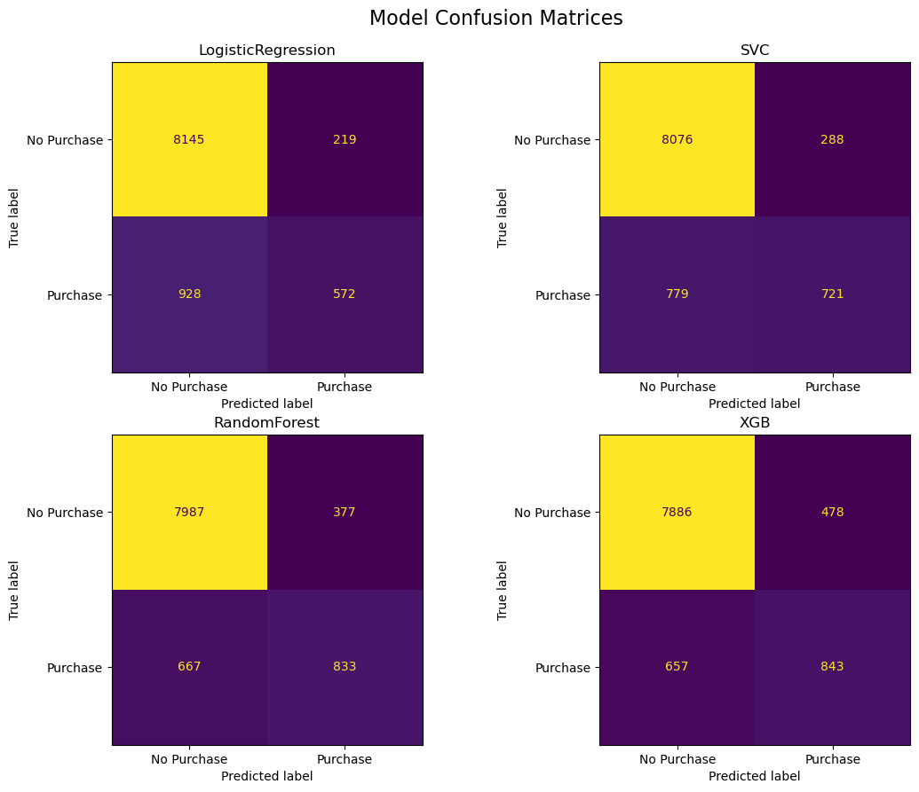
Fig.5 - Confusion Matrix for various models
From the confusion matrices above, we can see that the:
Logistic regression model is outputing 218 false positives, and 928 false negatives.
Support vector machine is outputing 288 false positives, and 779 false negatives.
Random forest is outputing 384 false positives, and 674 false negatives.
XGBoost model is outputing 478 false positives, and 657 false negatives.
Considering our goals of maximizing recall, with a budget of of 60% for precision, the Random forest and XGBoost model both look promising based on the confusion matrices.
Precision Recall Curves
We used sklearn’s cross_val_predict in combination with the PrecisionRecallDisplay.from_predictions method to generate Figure 6, which shows the precision recall curves for the models of interest.
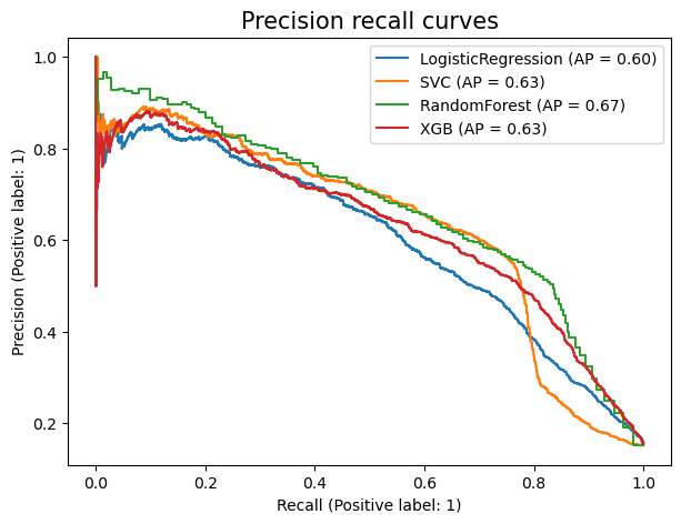
Fig.6 - Precision recall curve for various models
In assessing precision and recall curves, the following traits indicate a “better” curve:
A perfect curve would go from the top left of the plot, to the top right, and then to the bottom right. This would indicate a perfect scenario where a model can attain both 100% precision and recall (mostly impossible in real life)
A higher area under the curve
A higher average precision value (this is an average of the precision values at the different operating points in the curve and is shown in the legend as
AP)
Keeping the above points in mind, we can see that the Random forest and XGboost models appear to be able to generate our minimum budget of 60% precision while acheiving a 80% recall. We note that these curves have been generated with no hyperparameter tuning. In the model tuning section, we will determine if we need to manually set the operating point of our final model in order to increase or decrease a precision/recall score.
Model selected for further tuning
Above, we analyzed what can be considered to be “quick and dirty” models. This is the case since we simply fit these models to our pre-processed training data with no hyperparameter tuning, and then analyzed their results. The main purpose of training models in this fashion is to identify a promising model to tune further in order to solve our classification problem.
Based on these results alone, the Random forest and XGBoost models both appear to be promising. We note that both of these models are ensemble models, and share some similarities. As our dataset is not that large, we will select the Random forest model to tune further.
Finally, we note that Random forests are often a great model for classification problems as they inject randomness into a problem in the form of bagging and random features [Breiman, 2001].