Lecture 03: PCA applications class demo

import os
import random
import sys

import numpy as np
import pandas as pd

sys.path.append(os.path.join(os.path.abspath(".."), "code"))

import matplotlib.pyplot as plt
import seaborn as sns
from plotting_functions import *
from sklearn.decomposition import PCA
from sklearn.pipeline import make_pipeline
from sklearn.preprocessing import StandardScaler

plt.rcParams["font.size"] = 10
plt.rcParams["figure.figsize"] = (5, 4)
%matplotlib inline
pd.set_option("display.max_colwidth", 0)

PCA applications

There are tons of applications of PCA. In this section we’ll look at a few example applications.

Note

For this demo, we will be working with grayscale images. You can use PCA for coloured images as well. Just that it is a bit more work, as you have to apply it separately for each colour channel.

PCA for compression

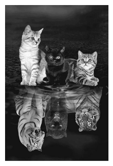
One way to think of PCA is that it’s a data compression algorithm. Let’s work through compressing a random image from the internet using PCA.

from matplotlib.pyplot import imread, imshow

# source: https://www.amazon.ca/Reflection-Needlework-Cross-Stitch-Embroidery-Decoration/dp/B08CCL7V2T
img = imread(os.path.join('../data/cats_reflection.jpg'))
plt.figure(figsize=[6,4])
plt.axis('off')
image_bw = img.sum(axis=2)/img.sum(axis=2).max()
print('dimensions:', image_bw.shape)
plt.imshow(image_bw, cmap=plt.cm.gray)
plt.show()

dimensions: (879, 580)

Let’s apply PCA with 40 components.

n_components=40
pca=PCA(n_components=n_components)
pca.fit(image_bw)

PCA(n_components=40)

In a Jupyter environment, please rerun this cell to show the HTML representation or trust the notebook.
On GitHub, the HTML representation is unable to render, please try loading this page with nbviewer.org.

We can examine the components.

pca.components_.shape

(40, 580)

We can also call SVD on our own and check whether the components of sklearn match with what’s returned by SVD.

image_bw_centered = image_bw - np.mean(image_bw, axis=0) # Let's center the image
U, S, Vt = np.linalg.svd(image_bw_centered, full_matrices=False)
U.shape, S.shape, Vt.shape

((879, 580), (580,), (580, 580))

Do the components given by sklearn match with the rows of Vt?

np.allclose(abs(pca.components_[0]), abs(Vt[0])) # taking abs because the solution is unique only upto sign

True

Let’s explore the component images created by the first few components: \(S_0U_0Vt_0 + S_1U_1Vt_1 + \dots + S_{8}U_{8}Vt_{8} + \dots\)

components = []
k = 10
for i in range(k):
    components.append(U[:, i][:, None]@Vt[i, :][None,:]) 

fig, axes = plt.subplots(2, 5, figsize=(14, 7), subplot_kw={"xticks": (), "yticks": ()})
for i, (component, ax) in enumerate(zip(components, axes.ravel())):
    if i==0:
        ax.imshow(image_bw, cmap=plt.cm.gray)
        ax.set_title('Original image')
    else:
        ax.imshow(component, cmap=plt.cm.gray)
        ax.set_title(f"{i-1}. component\nsingular value={np.round(S[i-1],2)}")
plt.show()

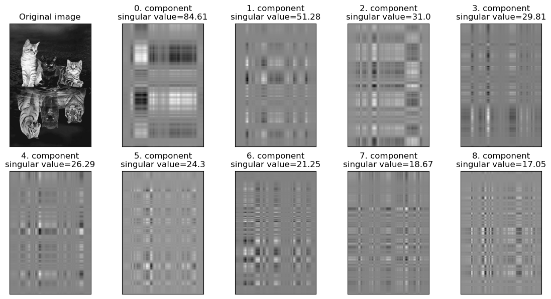
The first component with the largest singular value seems to be capturing the overall brightness and contrast and the subsequent components seem to be capturing more details such as textures and edges.

How good is the reconstruction with just 40 components?

Z_image = pca.transform(image_bw)
W_image = pca.components_
X_hat_image = pca.inverse_transform(Z_image)
plot_orig_compressed(image_bw, X_hat_image, n_components)

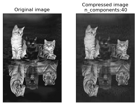
Pretty good reconstruction considering that we have only 40 components out of original 580 components.

Why is this compression?

• The size of the original matrix \(X\): ___

• The size of the matrices decomposed matrices \(U\), \(S\), and \(V^T\) after applying SVD: ___

• The size of the matrices \(U\), \(S\), and \(V^T\) after compression: ___

n, d = image_bw.shape[0], image_bw.shape[1]
n, d

(879, 580)

U.shape

(879, 580)

S.shape

(580,)

Vt.shape

(580, 580)

Let’s truncate for dimensionality reduction.

Z_svd = ((U[:, :n_components] * S[:n_components]))

Z_svd.shape

(879, 40)

W_svd = Vt[:n_components,:]

W_svd.shape

(40, 580)

orig_size = (n*d) # How many numbers do you need to store for the original image? 
orig_size

509820

# How many numbers do you need to store for the compressed image?
# n * n_components to store U 
# n_components to store S
# n_components*d to store Vt
compressed_size = (n*n_components) + n_components + (n_components*d) 
compressed_size

58400

PCA for feature extraction

An important application of PCA is feature extraction. Sometimes instead of using the raw data, it’s useful to come up with a more interpretable and compact representation of the data. For instance, in case of images, instead of looking at individual pixels, it’s useful to look at important components.

In Week 1, we clustered human face images, a small subset of Human Faces dataset (available here). We represented each image with feature vector extracted from pretrained CNNs. We got great clustering results but the feature vectors themselves were not very interpretable. Let’s examine whether we can do better with interpretation by applying a linear transformation using PCA.

import random
import os
import torch
from torchvision import datasets, models, transforms, utils
from PIL import Image
from torchvision import transforms

from torchvision.models import vgg16
import matplotlib.pyplot as plt

mpl.rcParams.update(mpl.rcParamsDefault)
plt.rcParams["image.cmap"] = "gray"

import torchvision

device = torch.device("cuda:0" if torch.cuda.is_available() else "cpu")

def set_seed(seed=42):
    torch.manual_seed(seed)
    np.random.seed(seed)
    random.seed(seed)

set_seed(seed=42)

import glob
IMAGE_SIZE = 200
def read_img_dataset(data_dir):     
    data_transforms = transforms.Compose(
        [
            transforms.Resize((IMAGE_SIZE, IMAGE_SIZE)), 
            transforms.Grayscale(num_output_channels=1),            
            transforms.ToTensor(),
            transforms.Lambda(torch.flatten)
        ])
               
    image_dataset = datasets.ImageFolder(root=data_dir, transform=data_transforms)
    dataloader = torch.utils.data.DataLoader(
         image_dataset, batch_size=BATCH_SIZE, shuffle=True, num_workers=0
    )
    dataset_size = len(image_dataset)
    class_names = image_dataset.classes
    inputs, classes = next(iter(dataloader))
    return inputs, classes

image_shape = (IMAGE_SIZE, IMAGE_SIZE)

def plot_sample_bw_imgs(inputs):
    fig, axes = plt.subplots(1, 5, figsize=(10, 8), subplot_kw={"xticks": (), "yticks": ()})
    for image, ax in zip(inputs, axes.ravel()):
        ax.imshow(image.reshape(image_shape))
    plt.show()

data_dir = "../data/people"
file_names = [image_file for image_file in glob.glob(data_dir + "/*/*.jpg")]
n_images = len(file_names)
BATCH_SIZE = n_images  # because our dataset is quite small
faces_inputs, classes = read_img_dataset(data_dir)

X_faces = faces_inputs.numpy()
X_faces.shape

(367, 40000)

X_faces[:24].shape

(24, 40000)

plot_sample_bw_imgs(X_faces[40:])

Let’s apply PCA on the data with n_components=100.

We’ll look at how to pick n_components in the next lecture.

n_components = 100
pca = PCA(n_components=100, random_state=123)
pca.fit(X_faces)

PCA(n_components=100, random_state=123)

In a Jupyter environment, please rerun this cell to show the HTML representation or trust the notebook.
On GitHub, the HTML representation is unable to render, please try loading this page with nbviewer.org.

How much variance are we covering with 100 components?

np.round(pca.explained_variance_ratio_, 3)

array([0.347, 0.098, 0.06 , 0.047, 0.038, 0.027, 0.025, 0.021, 0.019,
       0.015, 0.013, 0.013, 0.012, 0.01 , 0.008, 0.008, 0.007, 0.007,
       0.006, 0.006, 0.006, 0.005, 0.005, 0.005, 0.005, 0.004, 0.004,
       0.004, 0.004, 0.004, 0.004, 0.003, 0.003, 0.003, 0.003, 0.003,
       0.003, 0.003, 0.003, 0.002, 0.002, 0.002, 0.002, 0.002, 0.002,
       0.002, 0.002, 0.002, 0.002, 0.002, 0.002, 0.002, 0.002, 0.002,
       0.002, 0.002, 0.002, 0.002, 0.002, 0.001, 0.001, 0.001, 0.001,
       0.001, 0.001, 0.001, 0.001, 0.001, 0.001, 0.001, 0.001, 0.001,
       0.001, 0.001, 0.001, 0.001, 0.001, 0.001, 0.001, 0.001, 0.001,
       0.001, 0.001, 0.001, 0.001, 0.001, 0.001, 0.001, 0.001, 0.001,
       0.001, 0.001, 0.001, 0.001, 0.001, 0.001, 0.001, 0.001, 0.001,
       0.001], dtype=float32)

This is giving us variance covered by each component.

pca.explained_variance_ratio_.sum()

0.9410509

Z = pca.transform(X_faces)  # Transform the data
W = pca.components_  # principal components
X_hat = pca.inverse_transform(Z)  # reconstructions

What will be the shape of \(Z\), \(W\), and \(X_{hat}\)?

X_faces.shape 

(367, 40000)

Z.shape  

(367, 100)

W.shape

(100, 40000)

X_hat.shape

(367, 40000)

Components learned by PCA

W

array([[ 7.8977691e-03,  7.9017989e-03,  7.8920592e-03, ...,
         5.6139221e-03,  5.6564738e-03,  5.7036588e-03],
       [-7.3068761e-03, -7.4064992e-03, -7.5246757e-03, ...,
         4.7914064e-03,  4.6576657e-03,  4.5772959e-03],
       [-3.7232949e-04, -3.5709311e-04, -3.7663020e-04, ...,
        -4.2632208e-03, -4.2687790e-03, -4.1943062e-03],
       ...,
       [ 9.8374218e-04, -6.7102344e-05, -7.9967215e-04, ...,
        -2.0153911e-03, -7.3285995e-04, -4.0400025e-04],
       [ 4.9480475e-03,  4.8496895e-03,  4.7600521e-03, ...,
         1.0237189e-03,  1.2844147e-03,  1.5930103e-03],
       [-4.0721067e-04,  2.5537511e-04,  3.2496515e-05, ...,
         1.6387363e-03,  8.4129995e-04,  9.5578353e-04]], dtype=float32)

• We won’t quite be able to examine coefficients associated with all features and make sense of them because each feature in the original data just represents a pixel and there are a lot of them.

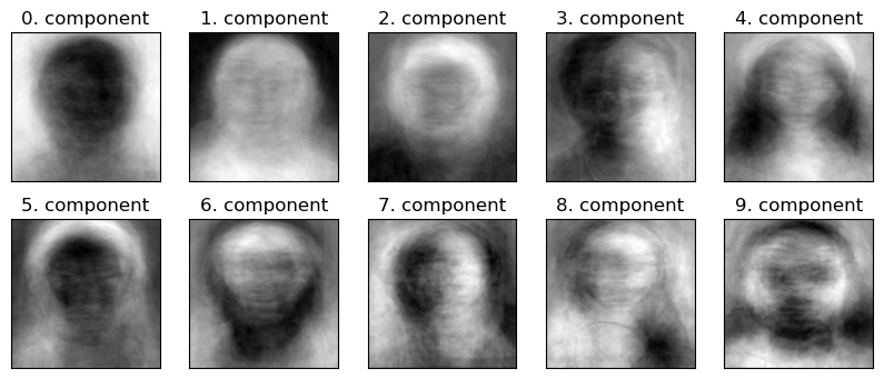
• But we can show principal components as images and can look for semantic themes in them.

• Let’s examine the first few components learned by PCA as images.

def plot_components(W): 
    fig, axes = plt.subplots(2, 5, figsize=(10, 4), subplot_kw={"xticks": (), "yticks": ()})
    for i, (component, ax) in enumerate(zip(W, axes.ravel())):
        ax.imshow(component.reshape(image_shape))
        ax.set_title("{}. component".format((i)))
    plt.show()    

plot_components(W)

• The components encode some semantic aspects of images.

• It’s not always easy to interpret what semantic aspect each component is roughly capturing but we could make some guesses.

• Component 0 is probably encoding the contrast between the background and the image, in particular, light background and darker face

• Component 1 is probably encoding lighter face and darker background.

Let’s examine some images where these components are strong.

for compn in [0, 1, 4]:
    plot_strong_comp_images(X_faces, Z, W, image_shape, compn=compn)

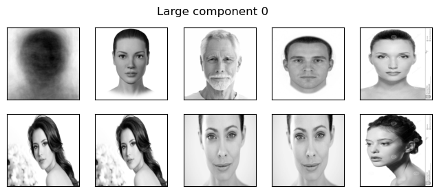
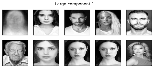
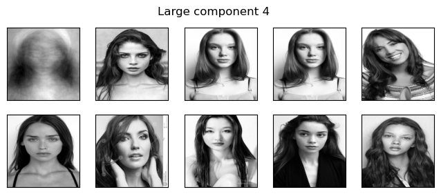
Looking at the sample images it does seem like:

• component 0 is capturing lighter background compared foreground

• component 1 is capturing darker background compared foreground

• component 4 is hard to interpret. Probably it’s capturing hairstyle, in particular, long hair on both sides?

Original images vs. Reconstructed images

• We can reconstruct the images from the transformed data \(Z\) and components \(W\).

• Let’s compare original images with the reconstructed images.

plot_orig_reconstructed_faces(X_faces[10:], X_hat[10:])

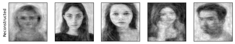
Decent reconstruction given that we are using only 100 components!!

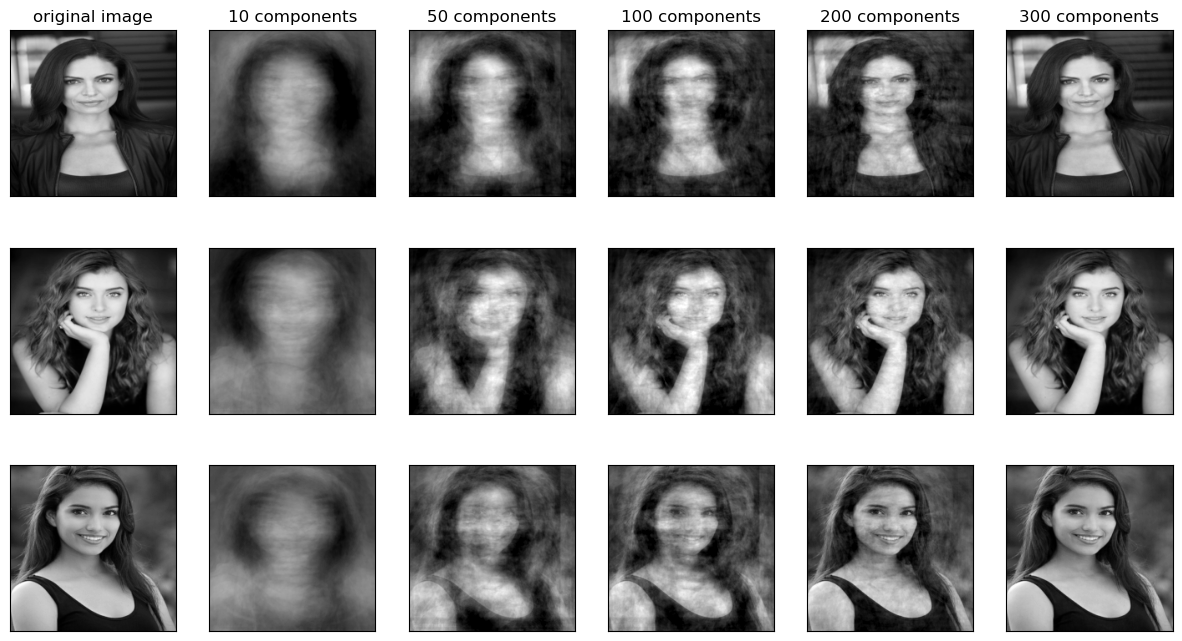
How many components?

• We can decide this based on how much variance is covered by how many components

• Or we can look at reconstruction of faces with varying number of components and pick \(k\) based on your application.

• Below we are reconstructing 3 faces with varying number of components in the range 10 to 300.

• As we can see, with 100 components, we are already capturing recognizable face (compared to 40,000 features in the original image).

plot_pca_faces(X_faces, image_shape, index=3)

If we fit PCA with n_components = 200 do you think the first 10 components would change in \(W\) compared to when we train it with n_components=100?

pca = PCA(n_components=200)
Z = pca.fit_transform(X_faces)
W = pca.components_

plot_components(W)

PCA for visualization

• One of the most common applications of PCA is visualizing high dimensional data.

• Suppose we want to visualize 20-dimensional countries of the world data.

• The dataset has country names linked to population, area size, GDP, literacy percentage, birthrate, mortality, net migration etc.

df = pd.read_csv("../data/countries of the world.csv")
df.head()

	Country	Region	Population	Area (sq. mi.)	Pop. Density (per sq. mi.)	Coastline (coast/area ratio)	Net migration	Infant mortality (per 1000 births)	GDP ($ per capita)	Literacy (%)	Phones (per 1000)	Arable (%)	Crops (%)	Other (%)	Climate	Birthrate	Deathrate	Agriculture	Industry	Service
0	Afghanistan	ASIA (EX. NEAR EAST)	31056997	647500	48,0	0,00	23,06	163,07	700.0	36,0	3,2	12,13	0,22	87,65	1	46,6	20,34	0,38	0,24	0,38
1	Albania	EASTERN EUROPE	3581655	28748	124,6	1,26	-4,93	21,52	4500.0	86,5	71,2	21,09	4,42	74,49	3	15,11	5,22	0,232	0,188	0,579
2	Algeria	NORTHERN AFRICA	32930091	2381740	13,8	0,04	-0,39	31	6000.0	70,0	78,1	3,22	0,25	96,53	1	17,14	4,61	0,101	0,6	0,298
3	American Samoa	OCEANIA	57794	199	290,4	58,29	-20,71	9,27	8000.0	97,0	259,5	10	15	75	2	22,46	3,27	NaN	NaN	NaN
4	Andorra	WESTERN EUROPE	71201	468	152,1	0,00	6,6	4,05	19000.0	100,0	497,2	2,22	0	97,78	3	8,71	6,25	NaN	NaN	NaN

df.info()

<class 'pandas.core.frame.DataFrame'>
RangeIndex: 227 entries, 0 to 226
Data columns (total 20 columns):
 #   Column                              Non-Null Count  Dtype  
---  ------                              --------------  -----  
 0   Country                             227 non-null    object 
 1   Region                              227 non-null    object 
 2   Population                          227 non-null    int64  
 3   Area (sq. mi.)                      227 non-null    int64  
 4   Pop. Density (per sq. mi.)          227 non-null    object 
 5   Coastline (coast/area ratio)        227 non-null    object 
 6   Net migration                       224 non-null    object 
 7   Infant mortality (per 1000 births)  224 non-null    object 
 8   GDP ($ per capita)                  226 non-null    float64
 9   Literacy (%)                        209 non-null    object 
 10  Phones (per 1000)                   223 non-null    object 
 11  Arable (%)                          225 non-null    object 
 12  Crops (%)                           225 non-null    object 
 13  Other (%)                           225 non-null    object 
 14  Climate                             205 non-null    object 
 15  Birthrate                           224 non-null    object 
 16  Deathrate                           223 non-null    object 
 17  Agriculture                         212 non-null    object 
 18  Industry                            211 non-null    object 
 19  Service                             212 non-null    object 
dtypes: float64(1), int64(2), object(17)
memory usage: 35.6+ KB

X_countries = df.drop(columns=["Country", "Region"])

Let’s replace commas with periods in columns with type object.

def convert_values(value):
    value = str(value)
    value = value.replace(",", ".")
    return float(value)


for col in X_countries.columns:
    if X_countries[col].dtype == object:
        X_countries[col] = X_countries[col].apply(convert_values)

X_countries.head()

	Population	Area (sq. mi.)	Pop. Density (per sq. mi.)	Coastline (coast/area ratio)	Net migration	Infant mortality (per 1000 births)	GDP ($ per capita)	Literacy (%)	Phones (per 1000)	Arable (%)	Crops (%)	Other (%)	Climate	Birthrate	Deathrate	Agriculture	Industry	Service
0	31056997	647500	48.0	0.00	23.06	163.07	700.0	36.0	3.2	12.13	0.22	87.65	1.0	46.60	20.34	0.380	0.240	0.380
1	3581655	28748	124.6	1.26	-4.93	21.52	4500.0	86.5	71.2	21.09	4.42	74.49	3.0	15.11	5.22	0.232	0.188	0.579
2	32930091	2381740	13.8	0.04	-0.39	31.00	6000.0	70.0	78.1	3.22	0.25	96.53	1.0	17.14	4.61	0.101	0.600	0.298
3	57794	199	290.4	58.29	-20.71	9.27	8000.0	97.0	259.5	10.00	15.00	75.00	2.0	22.46	3.27	NaN	NaN	NaN
4	71201	468	152.1	0.00	6.60	4.05	19000.0	100.0	497.2	2.22	0.00	97.78	3.0	8.71	6.25	NaN	NaN	NaN

• We have missing values

• The features are in different scales.

• Let’s create a pipeline with SimpleImputer and StandardScaler.

from sklearn.impute import SimpleImputer
n_components = 2
pipe = make_pipeline(SimpleImputer(), StandardScaler(), PCA(n_components=n_components))
pipe.fit(X_countries)
X_countries_pca = pipe.transform(X_countries)

print(
    "Variance Explained by the first %d principal components: %0.3f percent"
    % (n_components, sum(pipe.named_steps["pca"].explained_variance_ratio_) * 100)
)

Variance Explained by the first 2 principal components: 43.583 percent

• Good to know!

For each example, let’s get other information from the original data.

pca_df = pd.DataFrame(X_countries_pca, columns=["Z1", "Z2"], index=X_countries.index)
pca_df["Country"] = df["Country"]
pca_df["Population"] = X_countries["Population"]
pca_df["GDP"] = X_countries["GDP ($ per capita)"]
pca_df["Crops"] = X_countries["Crops (%)"]
pca_df["Infant mortality"] = X_countries["Infant mortality (per 1000 births)"]
pca_df["Birthrate"] = X_countries["Birthrate"]
pca_df["Literacy"] = X_countries["Literacy (%)"]
pca_df["Net migration"] = X_countries["Net migration"]
pca_df.fillna(pca_df["GDP"].mean(), inplace=True)
pca_df.head()

	Z1	Z2	Country	Population	GDP	Crops	Infant mortality	Birthrate	Literacy	Net migration
0	5.259255	-2.326683	Afghanistan	31056997	700.0	0.22	163.07	46.60	36.0	23.06
1	-0.260777	1.491964	Albania	3581655	4500.0	4.42	21.52	15.11	86.5	-4.93
2	1.154648	-1.904628	Algeria	32930091	6000.0	0.25	31.00	17.14	70.0	-0.39
3	-0.448853	2.255437	American Samoa	57794	8000.0	15.00	9.27	22.46	97.0	-20.71
4	-2.211518	-1.547689	Andorra	71201	19000.0	0.00	4.05	8.71	100.0	6.60

import plotly.express as px

fig = px.scatter(
    pca_df,
    x="Z1",
    y="Z2",
    color="Country",
    size="GDP",
    hover_data=[
        "Population",
        "Infant mortality",
        "Literacy",
        "Birthrate",
        "Net migration",
    ],
)
fig.show()

How to interpret the components?

• Each principal component has a coefficient associated with each feature in our original dataset.

• We can interpret the components by looking at the features with relatively bigger values (in magnitude) for coefficients for each components.

component_labels = ["PC " + str(i + 1) for i in range(n_components)]
W = pipe.named_steps["pca"].components_
plot_pca_w_vectors(W, component_labels, X_countries.columns)

Dimensionality reduction to reduce overfitting in supervised setting

• Often you would see dimensionality reduction being used as a preprocessing step in supervised learning setup.

• More features means higher possibility of overfitting.

• If we reduce number of dimensions, it may reduce overfitting and computational complexity.

Dimensionality reduction for anomaly detection

• A common application for dimensionality reduction is anomaly or outliers detection. For example:

  • Detecting fraud transactions.

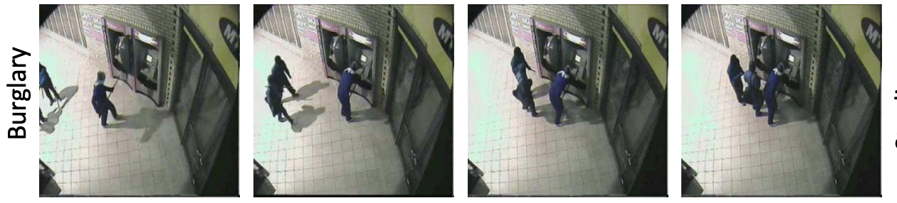
  • Detecting irregular activity in video frames.

  • It’s hard to find good anomaly detection datasets. A popular one is The KDD Cup ‘99 dataset.