Lecture 5: Class demo

Lecture 5: Class demo#

Imports#

# import the libraries
import os
import sys
sys.path.append(os.path.join(os.path.abspath(".."), (".."), "code"))
from plotting_functions import *
from utils import *

import matplotlib.pyplot as plt
import numpy as np
import pandas as pd

from sklearn.compose import ColumnTransformer, make_column_transformer
from sklearn.impute import SimpleImputer
from sklearn.model_selection import cross_val_score, cross_validate, train_test_split
from sklearn.neighbors import KNeighborsClassifier
from sklearn.pipeline import Pipeline, make_pipeline
from sklearn.preprocessing import OneHotEncoder, OrdinalEncoder, StandardScaler

%matplotlib inline

pd.set_option("display.max_colwidth", 200)

c = os.path.join(os.path.abspath(".."), (".."), "data/")
DATA_DIR = os.path.join(os.path.abspath(".."), (".."), "data/")
pd.set_option("display.max_colwidth", 200)

Data and splitting#

Do you recall the restaurants survey you completed at the start of the course?

Let’s use that data for this demo. You’ll find a wrangled version in the course repository.

df = pd.read_csv(DATA_DIR + 'cleaned_restaurant_data.csv')

df

	north_america	eat_out_freq	age	n_people	price	food_type	noise_level	good_server	comments	restaurant_name	target
0	Yes	3.0	29	10.0	120.0	Italian	medium	Yes	Ambience	NaN	dislike
1	Yes	2.0	23	3.0	20.0	Canadian/American	no music	No	food tastes bad	NaN	dislike
2	Yes	2.0	21	20.0	15.0	Chinese	medium	Yes	bad food	NaN	dislike
3	No	2.0	24	14.0	18.0	Other	medium	No	Overall vibe on the restaurant	NaN	dislike
4	Yes	5.0	23	30.0	20.0	Chinese	medium	Yes	A bad day	NaN	dislike
...	...	...	...	...	...	...	...	...	...	...	...
959	No	10.0	22	NaN	NaN	NaN	NaN	NaN	NaN	NaN	like
960	Yes	1.0	20	NaN	NaN	NaN	NaN	NaN	NaN	NaN	like
961	No	1.0	22	40.0	50.0	Chinese	medium	Yes	The self service sauce table is very clean and the sauces were always filled up.	Haidilao	like
962	Yes	3.0	21	NaN	NaN	NaN	NaN	NaN	NaN	NaN	like
963	Yes	3.0	27	20.0	22.0	Other	medium	Yes	Lots of meat that was very soft and tasty. Hearty and amazing broth. Good noodle thickness and consistency	Uno Beef Noodle	like

964 rows × 11 columns

df.describe()

	eat_out_freq	age	n_people	price
count	964.000000	964.000000	6.960000e+02	696.000000
mean	2.585187	23.975104	1.439254e+04	1472.179152
std	2.246486	4.556716	3.790481e+05	37903.575636
min	0.000000	10.000000	-2.000000e+00	0.000000
25%	1.000000	21.000000	1.000000e+01	18.000000
50%	2.000000	22.000000	2.000000e+01	25.000000
75%	3.000000	26.000000	3.000000e+01	40.000000
max	15.000000	46.000000	1.000000e+07	1000000.000000

Are there any unusual values in this data that you notice? Let’s get rid of these outliers.

upperbound_price = 200
lowerbound_people = 1
df = df[~(df['price'] > 200)]
restaurant_df = df[~(df['n_people'] < lowerbound_people)]
restaurant_df.shape

(942, 11)

restaurant_df.describe()

	eat_out_freq	age	n_people	price
count	942.000000	942.000000	674.000000	674.000000
mean	2.598057	23.992569	24.973294	34.023279
std	2.257787	4.582570	22.016660	29.018622
min	0.000000	10.000000	1.000000	0.000000
25%	1.000000	21.000000	10.000000	18.000000
50%	2.000000	22.000000	20.000000	25.000000
75%	3.000000	26.000000	30.000000	40.000000
max	15.000000	46.000000	200.000000	200.000000

We aim to predict whether a restaurant is liked or disliked.

# Separate `X` and `y`. 

X = restaurant_df.drop(columns=['target'])
y = restaurant_df['target']

Below I’m perturbing this data just to demonstrate a few concepts. Don’t do it in real life.

X.at[459, 'food_type'] = 'Quebecois'
X['price'] = X['price'] * 100

# Split the data
X_train, X_test, y_train, y_test = train_test_split(X, y, test_size=0.2, random_state=123)

Exploratory data analysis#

X_train.hist(bins=20, figsize=(12, 8));

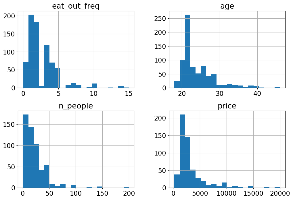
../../../_images/99d2c1fb4c2e5e045a61f60cd859c9c3dab605a936e6d34a4bb85f9d55c69eb1.png

Do you see anything interesting in these plots?

X_train['food_type'].value_counts()

food_type
Other                189
Canadian/American    131
Chinese              102
Indian                36
Italian               32
Thai                  20
Fusion                18
Mexican               17
fusion                 3
Quebecois              1
Name: count, dtype: int64

Error in data collection? Probably “Fusion” and “fusion” categories should be combined?

X_train['food_type'] = X_train['food_type'].replace("fusion", "Fusion")
X_test['food_type'] = X_test['food_type'].replace("fusion", "Fusion")

X_train['food_type'].value_counts()

food_type
Other                189
Canadian/American    131
Chinese              102
Indian                36
Italian               32
Fusion                21
Thai                  20
Mexican               17
Quebecois              1
Name: count, dtype: int64

Again, usually we should spend lots of time in EDA, but let’s stop here so that we have time to learn about transformers and pipelines.

Modeling#

Dummy Classifier#

from sklearn.dummy import DummyClassifier

dummy = DummyClassifier()
scores = cross_validate(dummy, X_train, y_train, return_train_score=True)
pd.DataFrame(scores)

	fit_time	score_time	test_score	train_score
0	0.000578	0.000353	0.516556	0.514950
1	0.000398	0.000337	0.516556	0.514950
2	0.000386	0.000255	0.516556	0.514950
3	0.000351	0.000240	0.513333	0.515755
4	0.000356	0.000249	0.513333	0.515755

We have a relatively balanced distribution of both ‘like’ and ‘dislike’ classes.

Let’s try KNN on this data#

Do you think KNN would work directly on X_train and y_train?

# Preprocessing and pipeline
from sklearn.neighbors import KNeighborsClassifier

knn = KNeighborsClassifier()
# knn.fit(X_train, y_train)

We need to preprocess the data before feeding it into machine learning models. What are the different types of features in the data?
What transformations are necessary before training a machine learning model?
Can we categorize features based on the type of transformations they require?

X_train[4:11]

	north_america	eat_out_freq	age	n_people	price	food_type	noise_level	good_server	comments	restaurant_name
62	Yes	2.0	24	20.0	3000.0	Indian	high	Yes	bad taste	east is east
694	No	0.0	20	NaN	NaN	NaN	NaN	NaN	NaN	NaN
890	No	5.0	21	50.0	3500.0	Canadian/American	high	Yes	5	Joeys Shipyards
677	Yes	3.0	20	30.0	2000.0	Mexican	low	Yes	NaN	NaN
161	No	0.0	27	NaN	NaN	NaN	NaN	NaN	NaN	NaN
571	Yes	3.0	22	NaN	NaN	NaN	NaN	NaN	NaN	NaN
11	Yes	2.0	21	30.0	3000.0	Chinese	medium	Yes	food that didn't come	Happy Lamb

numeric_feats = ['age', 'n_people', 'price'] # Continuous and quantitative features
categorical_feats = ['food_type', 'north_america'] # Discrete and qualitative features
binary_feats = ['good_server'] # Categorical features with only two possible values 
ordinal_feats = ['noise_level'] # Some natural ordering in the categories 
noise_cats = ['no music', 'low', 'medium', 'high', 'crazy loud']
drop_feats = ['comments', 'restaurant_name', 'eat_out_freq'] # Dropping text feats and `eat_out_freq` because it's not that useful

X_train.columns

Index(['north_america', 'eat_out_freq', 'age', 'n_people', 'price',
       'food_type', 'noise_level', 'good_server', 'comments',
       'restaurant_name'],
      dtype='object')

X_train['food_type'].value_counts()

food_type
Other                189
Canadian/American    131
Chinese              102
Indian                36
Italian               32
Fusion                21
Thai                  20
Mexican               17
Quebecois              1
Name: count, dtype: int64

X_train['north_america'].value_counts()

north_america
Yes                    415
No                     330
Don't want to share      8
Name: count, dtype: int64

X_train['good_server'].value_counts()

good_server
Yes    396
No     148
Name: count, dtype: int64

X_train['noise_level'].value_counts()

noise_level
medium        232
low           186
high           75
no music       37
crazy loud     18
Name: count, dtype: int64

Let’s begin with numeric features. What if we just use numeric features to train a KNN model? Would it work?

X_train_num = X_train[numeric_feats]
X_test_num = X_test[numeric_feats]
# knn.fit(X_train_num, y_train)

We need to deal with NaN values.

sklearn’s `SimpleImputer`#

# Impute numeric features using SimpleImputer
from sklearn.impute import SimpleImputer

imputer = SimpleImputer(strategy='median')

# fit the imputer 
imputer.fit(X_train_num)

# Transform training data 
X_train_num_imp = imputer.transform(X_train_num)

# Transform test data 
X_test_num_imp = imputer.transform(X_test_num)

knn.fit(X_train_num_imp, y_train)

KNeighborsClassifier()

In a Jupyter environment, please rerun this cell to show the HTML representation or trust the notebook.
On GitHub, the HTML representation is unable to render, please try loading this page with nbviewer.org.

No more errors. It worked! Let’s try cross validation.

knn.score(X_train_num_imp, y_train)

0.6706507304116865

knn.score(X_test_num_imp, y_test)

0.49206349206349204

We have slightly improved results in comparison to the dummy model.

Discussion questions#

What’s the difference between sklearn estimators and transformers?
Can you think of a better way to impute missing values?

Do we need to scale the data?

X_train[numeric_feats]

	age	n_people	price
80	21	30.0	2200.0
934	21	30.0	3000.0
911	20	40.0	2500.0
459	21	NaN	NaN
62	24	20.0	3000.0
...	...	...	...
106	27	10.0	1500.0
333	24	12.0	800.0
393	20	5.0	1500.0
376	20	NaN	NaN
525	20	50.0	3000.0

753 rows × 3 columns

# Scale the imputed data 

from sklearn.preprocessing import StandardScaler
scaler = StandardScaler()
scaler.fit(X_train_num_imp)
X_train_num_imp_scaled = scaler.transform(X_train_num_imp)
X_test_num_imp_scaled = scaler.transform(X_test_num_imp)

Alternative methods for scaling#

MinMaxScaler: Transform each feature to a desired range
RobustScaler: Scale features using median and quantiles. Robust to outliers.
Normalizer: Works on rows rather than columns. Normalize examples individually to unit norm.
MaxAbsScaler: A scaler that scales each feature by its maximum absolute value.
- What would happen when you apply StandardScaler to sparse data?
You can also apply custom scaling on columns using FunctionTransformer. For example, when a column follows the power law distribution (a handful of your values have many data points whereas most other values have few data points) log scaling is helpful.

For now, let’s focus on StandardScaler. Let’s carry out cross-validation

cross_val_score(knn, X_train_num_imp_scaled, y_train)

array([0.55629139, 0.49006623, 0.56953642, 0.54      , 0.53333333])

In this case, we don’t see a big difference with StandardScaler. But usually, scaling is a good idea.

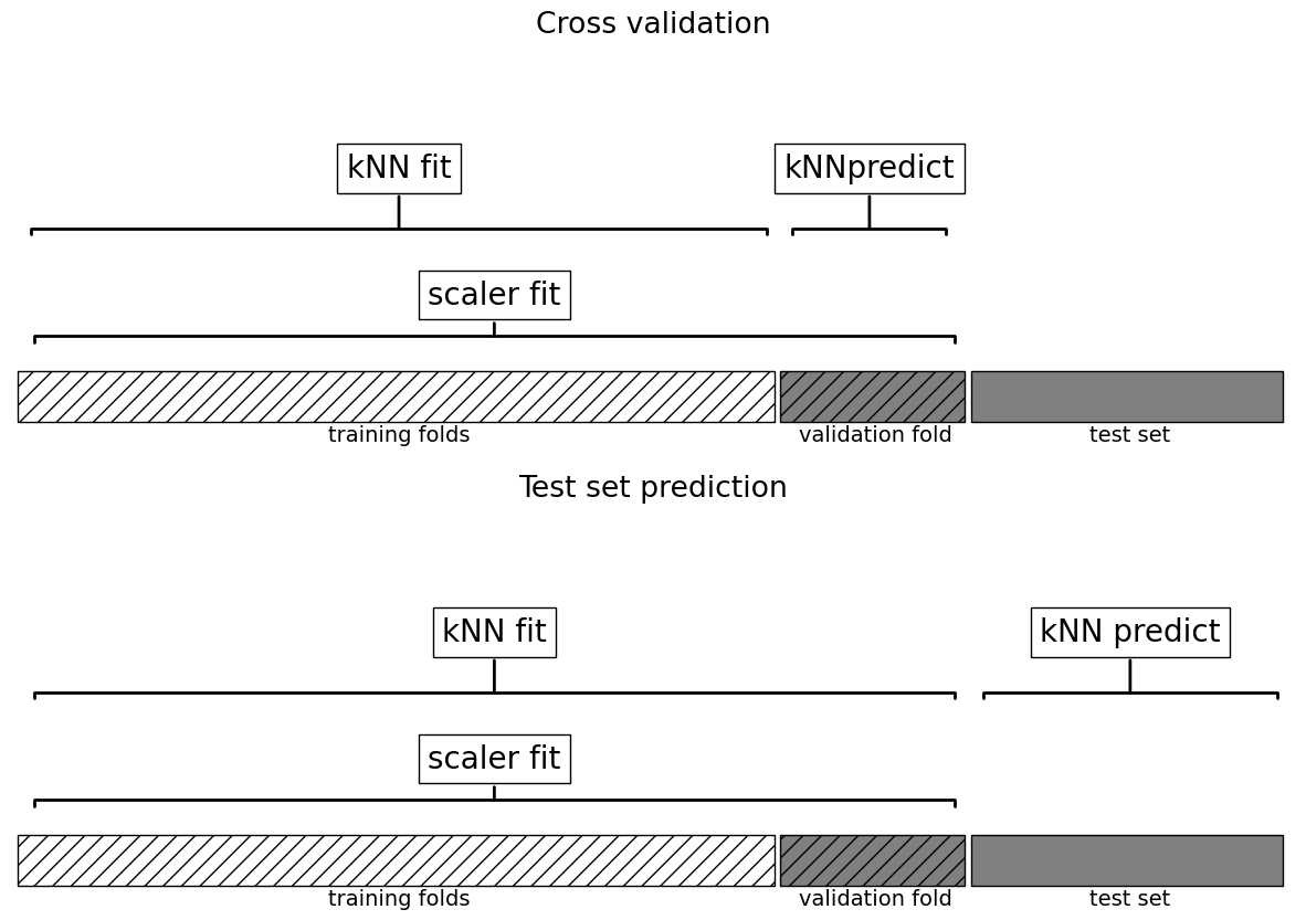
This worked but are we doing anything wrong here?
What’s the problem with calling cross_val_score with preprocessed data?

plot_improper_processing("kNN")

../../../_images/abcd4de550957df772d666bba48eee9268f66804183b87bf60bced0bb88225db.png

How would you do it properly? Enter sklearn pipelines!!#

# Create a pipeline 
pipe_knn = make_pipeline(
    SimpleImputer(strategy="median"),
    StandardScaler(), 
    KNeighborsClassifier()
) 

cross_val_score(pipe_knn, X_train_num, y_train).mean()

np.float64(0.5245916114790287)

What is happening under the hood?
Why is this a better approach?

Source

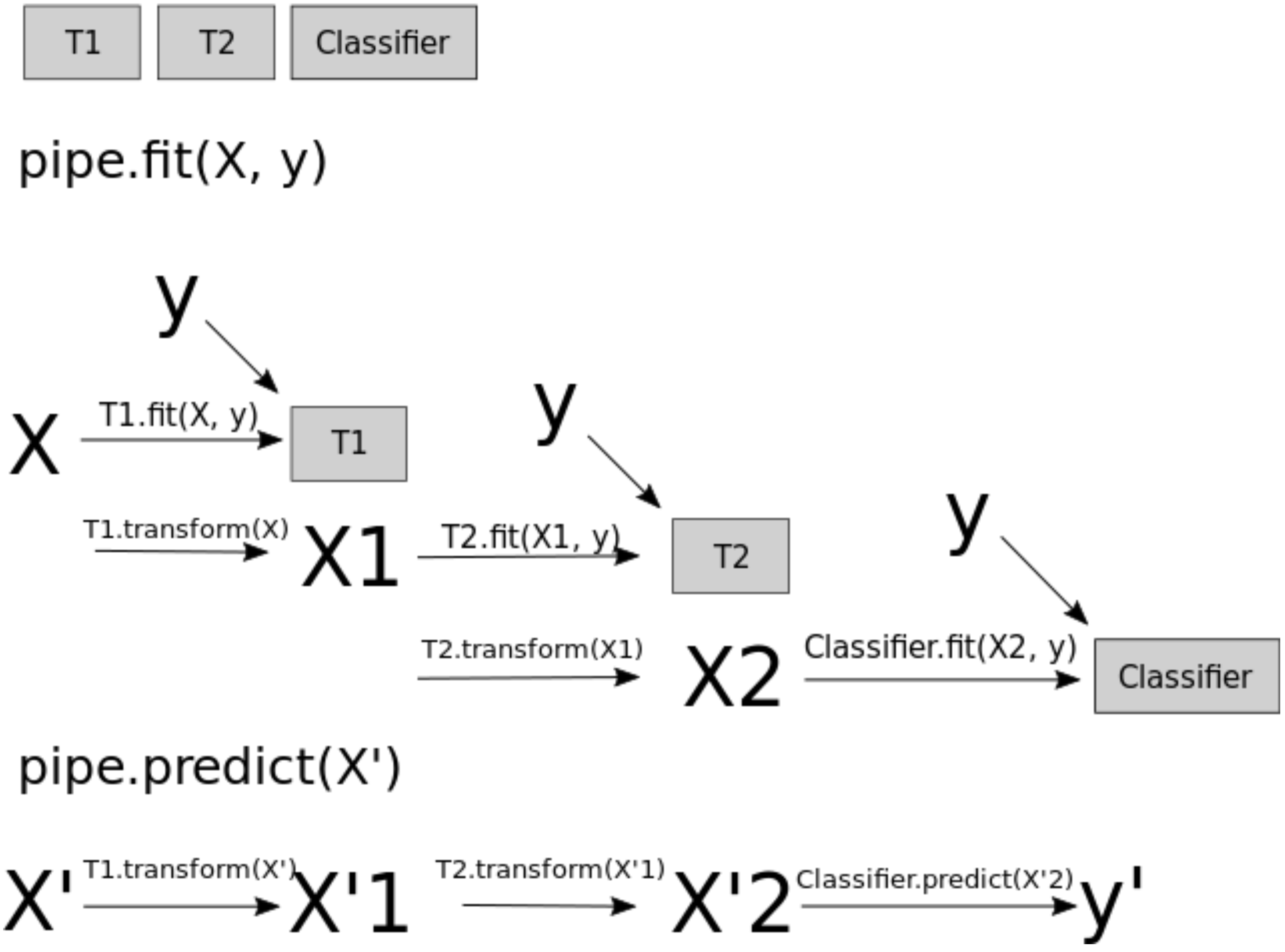
plot_proper_processing("kNN")

../../../_images/957abbb4f456c4c15742a17d8e5f9762f532bfc34682b198bff7cb60d0e7f81d.png

Categorical features#

Let’s assess the scores using categorical features.

X_train['food_type'].value_counts()

food_type
Other                189
Canadian/American    131
Chinese              102
Indian                36
Italian               32
Fusion                21
Thai                  20
Mexican               17
Quebecois              1
Name: count, dtype: int64

X_train[categorical_feats]

	food_type	north_america
80	Chinese	No
934	Canadian/American	Yes
911	Canadian/American	No
459	Quebecois	Yes
62	Indian	Yes
...	...	...
106	Chinese	No
333	Other	No
393	Canadian/American	Yes
376	NaN	Yes
525	Chinese	Don't want to share

753 rows × 2 columns

X_train['north_america'].value_counts()

north_america
Yes                    415
No                     330
Don't want to share      8
Name: count, dtype: int64

X_train['food_type'].value_counts()

food_type
Other                189
Canadian/American    131
Chinese              102
Indian                36
Italian               32
Fusion                21
Thai                  20
Mexican               17
Quebecois              1
Name: count, dtype: int64

X_train_cat = X_train[categorical_feats]
X_test_cat = X_test[categorical_feats]

# One-hot encoding of categorical features 
from sklearn.preprocessing import OneHotEncoder
# Create class object
ohe = OneHotEncoder(sparse_output=False)

# fit OneHotEncoder
ohe.fit(X_train_cat, y_train)

X_train_cat_ohe  = ohe.transform(X_train_cat)# transform the train set
X_test_cat_ohe  =  ohe.transform(X_test_cat)# transform the test set

X_train_cat_ohe

array([[0., 1., 0., ..., 0., 1., 0.],
       [1., 0., 0., ..., 0., 0., 1.],
       [1., 0., 0., ..., 0., 1., 0.],
       ...,
       [1., 0., 0., ..., 0., 0., 1.],
       [0., 0., 0., ..., 0., 0., 1.],
       [0., 1., 0., ..., 1., 0., 0.]])

It’s a sparse matrix.
Why? What would happen if we pass sparse_output=False? Why we might want to do that?

# Get the OHE feature names 

ohe_feats = ohe.get_feature_names_out().tolist()
ohe_feats

['food_type_Canadian/American',
 'food_type_Chinese',
 'food_type_Fusion',
 'food_type_Indian',
 'food_type_Italian',
 'food_type_Mexican',
 'food_type_Other',
 'food_type_Quebecois',
 'food_type_Thai',
 'food_type_nan',
 "north_america_Don't want to share",
 'north_america_No',
 'north_america_Yes']

pd.DataFrame(X_train_cat_ohe, columns = ohe_feats)

	food_type_Canadian/American	food_type_Chinese	food_type_Fusion	food_type_Indian	food_type_Italian	food_type_Mexican	food_type_Other	food_type_Quebecois	food_type_Thai	food_type_nan	north_america_Don't want to share	north_america_No	north_america_Yes
0	0.0	1.0	0.0	0.0	0.0	0.0	0.0	0.0	0.0	0.0	0.0	1.0	0.0
1	1.0	0.0	0.0	0.0	0.0	0.0	0.0	0.0	0.0	0.0	0.0	0.0	1.0
2	1.0	0.0	0.0	0.0	0.0	0.0	0.0	0.0	0.0	0.0	0.0	1.0	0.0
3	0.0	0.0	0.0	0.0	0.0	0.0	0.0	1.0	0.0	0.0	0.0	0.0	1.0
4	0.0	0.0	0.0	1.0	0.0	0.0	0.0	0.0	0.0	0.0	0.0	0.0	1.0
...	...	...	...	...	...	...	...	...	...	...	...	...	...
748	0.0	1.0	0.0	0.0	0.0	0.0	0.0	0.0	0.0	0.0	0.0	1.0	0.0
749	0.0	0.0	0.0	0.0	0.0	0.0	1.0	0.0	0.0	0.0	0.0	1.0	0.0
750	1.0	0.0	0.0	0.0	0.0	0.0	0.0	0.0	0.0	0.0	0.0	0.0	1.0
751	0.0	0.0	0.0	0.0	0.0	0.0	0.0	0.0	0.0	1.0	0.0	0.0	1.0
752	0.0	1.0	0.0	0.0	0.0	0.0	0.0	0.0	0.0	0.0	1.0	0.0	0.0

753 rows × 13 columns

cross_val_score(knn, X_train_cat_ohe, y_train)

array([0.54304636, 0.52980132, 0.55629139, 0.54666667, 0.55333333])

What’s wrong here?
How can we fix this?

Let’s do this properly with a pipeline.

# Code to create a pipeline for OHE and KNN
pipe_ohe_knn = make_pipeline(
    OneHotEncoder(sparse_output=False, handle_unknown="ignore"),
    KNeighborsClassifier()
)

cross_val_score(pipe_ohe_knn, X_train_cat, y_train)

array([0.54304636, 0.52980132, 0.55629139, 0.54666667, 0.55333333])

Ordinal features#

Let’s examine the scores using ordinal features.

noise_ordering = ['no music', 'low', 'medium', 'high', 'crazy loud']

X_train['noise_level'].value_counts()

noise_level
medium        232
low           186
high           75
no music       37
crazy loud     18
Name: count, dtype: int64

X_train['noise_level'].isnull().any()

np.True_

There are missing values. So we need an imputer.

from sklearn.preprocessing import OrdinalEncoder
noise_ordering = ['no music', 'low', 'medium', 'high', 'crazy loud']

pipe_ordinal_knn = make_pipeline(
    SimpleImputer(strategy="most_frequent"),
    OrdinalEncoder(categories=[noise_ordering]),
    KNeighborsClassifier()
)

cross_val_score(pipe_ordinal_knn, X_train[['noise_level']], y_train)

array([0.54966887, 0.56953642, 0.57615894, 0.48666667, 0.56666667])

Right now we are working with numeric and categorical features separately. But ideally when we create a model, we need to use all these features together.

Enter column transformer!

How can we horizontally stack

preprocessed numeric features,
preprocessed binary features,
preprocessed ordinal features, and
preprocessed categorical features?

Let’s define a column transformer.

from sklearn.compose import make_column_transformer

numeric_transformer = make_pipeline(SimpleImputer(strategy="median"),
                                    StandardScaler()) 
binary_transformer = make_pipeline(SimpleImputer(strategy="most_frequent"), 
                                    OneHotEncoder(drop="if_binary"))
ordinal_transformer = make_pipeline(SimpleImputer(strategy="most_frequent"), 
                                    OrdinalEncoder(categories=[noise_ordering]))
categorical_transformer = make_pipeline(SimpleImputer(strategy="most_frequent"), 
                                        OneHotEncoder(sparse_output=False, 
                                                  handle_unknown="ignore"))

# Define the column transformer
preprocessor = make_column_transformer(
    (numeric_transformer, numeric_feats),
    (binary_transformer, binary_feats),
    (ordinal_transformer, ordinal_feats),
    (categorical_transformer, categorical_feats),
    ("drop", drop_feats)    
)

How does the transformed data look like?

categorical_feats

['food_type', 'north_america']

X_train.shape

(753, 10)

transformed = preprocessor.fit_transform(X_train)
transformed.shape

(753, 17)

# Getting feature names from a column transformer
ohe_feat_names = preprocessor.named_transformers_['pipeline-4']['onehotencoder'].get_feature_names_out(categorical_feats).tolist()
ohe_feat_names

['food_type_Canadian/American',
 'food_type_Chinese',
 'food_type_Fusion',
 'food_type_Indian',
 'food_type_Italian',
 'food_type_Mexican',
 'food_type_Other',
 'food_type_Quebecois',
 'food_type_Thai',
 "north_america_Don't want to share",
 'north_america_No',
 'north_america_Yes']

numeric_feats

['age', 'n_people', 'price']

feat_names = numeric_feats + binary_feats + ordinal_feats + ohe_feat_names

transformed

array([[-0.66941678,  0.31029469, -0.36840629, ...,  0.        ,
         1.        ,  0.        ],
       [-0.66941678,  0.31029469, -0.05422496, ...,  0.        ,
         0.        ,  1.        ],
       [-0.89515383,  0.82336432, -0.25058829, ...,  0.        ,
         1.        ,  0.        ],
       ...,
       [-0.89515383, -0.97237936, -0.64331495, ...,  0.        ,
         0.        ,  1.        ],
       [-0.89515383, -0.20277493, -0.25058829, ...,  0.        ,
         0.        ,  1.        ],
       [-0.89515383,  1.33643394, -0.05422496, ...,  1.        ,
         0.        ,  0.        ]])

You can also get feature names of the transformed data directly from the column transformer object.

feat_names = preprocessor.get_feature_names_out()

We have new columns for the categorical features. Let’s create a pipeline with the preprocessor and SVC.

pd.DataFrame(transformed, columns = feat_names)

	pipeline-1__age	pipeline-1__n_people	pipeline-1__price	pipeline-2__good_server_Yes	pipeline-3__noise_level	pipeline-4__food_type_Canadian/American	pipeline-4__food_type_Chinese	pipeline-4__food_type_Fusion	pipeline-4__food_type_Indian	pipeline-4__food_type_Italian	pipeline-4__food_type_Mexican	pipeline-4__food_type_Other	pipeline-4__food_type_Quebecois	pipeline-4__food_type_Thai	pipeline-4__north_america_Don't want to share	pipeline-4__north_america_No	pipeline-4__north_america_Yes
0	-0.669417	0.310295	-0.368406	0.0	3.0	0.0	1.0	0.0	0.0	0.0	0.0	0.0	0.0	0.0	0.0	1.0	0.0
1	-0.669417	0.310295	-0.054225	1.0	1.0	1.0	0.0	0.0	0.0	0.0	0.0	0.0	0.0	0.0	0.0	0.0	1.0
2	-0.895154	0.823364	-0.250588	1.0	2.0	1.0	0.0	0.0	0.0	0.0	0.0	0.0	0.0	0.0	0.0	1.0	0.0
3	-0.669417	-0.202775	-0.250588	1.0	2.0	0.0	0.0	0.0	0.0	0.0	0.0	0.0	1.0	0.0	0.0	0.0	1.0
4	0.007794	-0.202775	-0.054225	1.0	3.0	0.0	0.0	0.0	1.0	0.0	0.0	0.0	0.0	0.0	0.0	0.0	1.0
...	...	...	...	...	...	...	...	...	...	...	...	...	...	...	...	...	...
748	0.685006	-0.715845	-0.643315	1.0	2.0	0.0	1.0	0.0	0.0	0.0	0.0	0.0	0.0	0.0	0.0	1.0	0.0
749	0.007794	-0.613231	-0.918224	1.0	2.0	0.0	0.0	0.0	0.0	0.0	0.0	1.0	0.0	0.0	0.0	1.0	0.0
750	-0.895154	-0.972379	-0.643315	0.0	1.0	1.0	0.0	0.0	0.0	0.0	0.0	0.0	0.0	0.0	0.0	0.0	1.0
751	-0.895154	-0.202775	-0.250588	1.0	2.0	0.0	0.0	0.0	0.0	0.0	0.0	1.0	0.0	0.0	0.0	0.0	1.0
752	-0.895154	1.336434	-0.054225	1.0	3.0	0.0	1.0	0.0	0.0	0.0	0.0	0.0	0.0	0.0	1.0	0.0	0.0

753 rows × 17 columns

from sklearn.svm import SVC 

svc_all_pipe = make_pipeline(preprocessor, SVC()) # create a pipeline with column transformer. 
cross_val_score(svc_all_pipe, X_train, y_train).mean()

np.float64(0.686569536423841)

We are getting better results!

	food_type_Canadian/American	food_type_Chinese	food_type_Fusion	food_type_Indian	food_type_Italian	food_type_Mexican	food_type_Other	food_type_Quebecois	food_type_Thai	food_type_nan	north_america_Don't want to share	north_america_No	north_america_Yes
0	0.0	1.0	0.0	0.0	0.0	0.0	0.0	0.0	0.0	0.0	0.0	1.0	0.0
1	1.0	0.0	0.0	0.0	0.0	0.0	0.0	0.0	0.0	0.0	0.0	0.0	1.0
2	1.0	0.0	0.0	0.0	0.0	0.0	0.0	0.0	0.0	0.0	0.0	1.0	0.0
3	0.0	0.0	0.0	0.0	0.0	0.0	0.0	1.0	0.0	0.0	0.0	0.0	1.0
4	0.0	0.0	0.0	1.0	0.0	0.0	0.0	0.0	0.0	0.0	0.0	0.0	1.0
...	...	...	...	...	...	...	...	...	...	...	...	...	...
748	0.0	1.0	0.0	0.0	0.0	0.0	0.0	0.0	0.0	0.0	0.0	1.0	0.0
749	0.0	0.0	0.0	0.0	0.0	0.0	1.0	0.0	0.0	0.0	0.0	1.0	0.0
750	1.0	0.0	0.0	0.0	0.0	0.0	0.0	0.0	0.0	0.0	0.0	0.0	1.0
751	0.0	0.0	0.0	0.0	0.0	0.0	0.0	0.0	0.0	1.0	0.0	0.0	1.0
752	0.0	1.0	0.0	0.0	0.0	0.0	0.0	0.0	0.0	0.0	1.0	0.0	0.0

	food_type_Canadian/American	food_type_Chinese	food_type_Fusion	food_type_Indian	food_type_Italian	food_type_Mexican	food_type_Other	food_type_Quebecois	food_type_Thai	food_type_nan	north_america_Don't want to share	north_america_No	north_america_Yes
0	0.0	1.0	0.0	0.0	0.0	0.0	0.0	0.0	0.0	0.0	0.0	1.0	0.0
1	1.0	0.0	0.0	0.0	0.0	0.0	0.0	0.0	0.0	0.0	0.0	0.0	1.0
2	1.0	0.0	0.0	0.0	0.0	0.0	0.0	0.0	0.0	0.0	0.0	1.0	0.0
3	0.0	0.0	0.0	0.0	0.0	0.0	0.0	1.0	0.0	0.0	0.0	0.0	1.0
4	0.0	0.0	0.0	1.0	0.0	0.0	0.0	0.0	0.0	0.0	0.0	0.0	1.0
...	...	...	...	...	...	...	...	...	...	...	...	...	...
748	0.0	1.0	0.0	0.0	0.0	0.0	0.0	0.0	0.0	0.0	0.0	1.0	0.0
749	0.0	0.0	0.0	0.0	0.0	0.0	1.0	0.0	0.0	0.0	0.0	1.0	0.0
750	1.0	0.0	0.0	0.0	0.0	0.0	0.0	0.0	0.0	0.0	0.0	0.0	1.0
751	0.0	0.0	0.0	0.0	0.0	0.0	0.0	0.0	0.0	1.0	0.0	0.0	1.0
752	0.0	1.0	0.0	0.0	0.0	0.0	0.0	0.0	0.0	0.0	1.0	0.0	0.0