
Lectures 6: Class demo#
Imports#
import os
import sys

sys.path.append(os.path.join(os.path.abspath(".."), (".."), "code"))

import matplotlib.pyplot as plt
import mglearn
import numpy as np
import pandas as pd
from plotting_functions import *
from sklearn.dummy import DummyClassifier
from sklearn.impute import SimpleImputer
from sklearn.model_selection import cross_val_score, cross_validate, train_test_split
from sklearn.pipeline import Pipeline, make_pipeline
from sklearn.preprocessing import OneHotEncoder, StandardScaler
from sklearn.svm import SVC
from sklearn.tree import DecisionTreeClassifier
from utils import *

%matplotlib inline
pd.set_option("display.max_colwidth", 200)
DATA_DIR = os.path.join(os.path.abspath(".."), (".."), "data/")
from sklearn import set_config

set_config(display="diagram")
Let’s look at an example of tuning max_depth of the DecisionTreeClassifier on the Spotify dataset.
spotify_df = pd.read_csv(DATA_DIR + "spotify.csv", index_col=0)
X_spotify = spotify_df.drop(columns=["target", "artist"])
y_spotify = spotify_df["target"]
X_spotify.head()
| acousticness | danceability | duration_ms | energy | instrumentalness | key | liveness | loudness | mode | speechiness | tempo | time_signature | valence | song_title | |
|---|---|---|---|---|---|---|---|---|---|---|---|---|---|---|
| 0 | 0.0102 | 0.833 | 204600 | 0.434 | 0.021900 | 2 | 0.1650 | -8.795 | 1 | 0.4310 | 150.062 | 4.0 | 0.286 | Mask Off |
| 1 | 0.1990 | 0.743 | 326933 | 0.359 | 0.006110 | 1 | 0.1370 | -10.401 | 1 | 0.0794 | 160.083 | 4.0 | 0.588 | Redbone |
| 2 | 0.0344 | 0.838 | 185707 | 0.412 | 0.000234 | 2 | 0.1590 | -7.148 | 1 | 0.2890 | 75.044 | 4.0 | 0.173 | Xanny Family |
| 3 | 0.6040 | 0.494 | 199413 | 0.338 | 0.510000 | 5 | 0.0922 | -15.236 | 1 | 0.0261 | 86.468 | 4.0 | 0.230 | Master Of None |
| 4 | 0.1800 | 0.678 | 392893 | 0.561 | 0.512000 | 5 | 0.4390 | -11.648 | 0 | 0.0694 | 174.004 | 4.0 | 0.904 | Parallel Lines |
X_train, X_test, y_train, y_test = train_test_split(
    X_spotify, y_spotify, test_size=0.2, random_state=123
)
numeric_feats = ['acousticness', 'danceability', 'energy',
                 'instrumentalness', 'liveness', 'loudness',
                 'speechiness', 'tempo', 'valence']
categorical_feats = ['time_signature', 'key']
passthrough_feats = ['mode']
text_feat = "song_title"
from sklearn.compose import make_column_transformer
from sklearn.feature_extraction.text import CountVectorizer

preprocessor = make_column_transformer(
    (StandardScaler(), numeric_feats),
    (OneHotEncoder(handle_unknown = "ignore"), categorical_feats),
    ("passthrough", passthrough_feats),
    (CountVectorizer(max_features=100, stop_words="english"), text_feat)
)

svc_pipe = make_pipeline(preprocessor, SVC)
What’s the general approach for model selection?
mglearn.plots.plot_grid_search_overview()
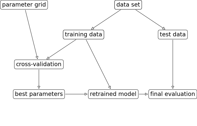
Hyperparameter optimization is so common that sklearn includes two classes to automate these steps.
Exhaustive grid search:
sklearn.model_selection.GridSearchCVRandomized search:
sklearn.model_selection.RandomizedSearchCV
The “CV” stands for cross-validation; these methods have built-in cross-validation.
Exhaustive grid search: sklearn.model_selection.GridSearchCV#
For
GridSearchCVwe needan instantiated model or a pipeline
a parameter grid: A user specifies a set of values for each hyperparameter.
other optional arguments
The method considers product of the sets and evaluates each combination one by one.
preprocessor.fit(X_train)
ColumnTransformer(transformers=[('standardscaler', StandardScaler(),
                                 ['acousticness', 'danceability', 'energy',
                                  'instrumentalness', 'liveness', 'loudness',
                                  'speechiness', 'tempo', 'valence']),
                                ('onehotencoder',
                                 OneHotEncoder(handle_unknown='ignore'),
                                 ['time_signature', 'key']),
                                ('passthrough', 'passthrough', ['mode']),
                                ('countvectorizer',
                                 CountVectorizer(max_features=100,
                                                 stop_words='english'),
                                 'song_title')])
In a Jupyter environment, please rerun this cell to show the HTML representation or trust the notebook. On GitHub, the HTML representation is unable to render, please try loading this page with nbviewer.org.
ColumnTransformer(transformers=[('standardscaler', StandardScaler(),
                                 ['acousticness', 'danceability', 'energy',
                                  'instrumentalness', 'liveness', 'loudness',
                                  'speechiness', 'tempo', 'valence']),
                                ('onehotencoder',
                                 OneHotEncoder(handle_unknown='ignore'),
                                 ['time_signature', 'key']),
                                ('passthrough', 'passthrough', ['mode']),
                                ('countvectorizer',
                                 CountVectorizer(max_features=100,
                                                 stop_words='english'),
'song_title')])['acousticness', 'danceability', 'energy', 'instrumentalness', 'liveness', 'loudness', 'speechiness', 'tempo', 'valence']
StandardScaler()
['time_signature', 'key']
OneHotEncoder(handle_unknown='ignore')
['mode']
passthrough
song_title
CountVectorizer(max_features=100, stop_words='english')
from sklearn.model_selection import GridSearchCV

pipe_svm = make_pipeline(preprocessor, SVC())

param_grid = {
    "columntransformer__countvectorizer__max_features": [100, 200, 400, 800, 1000, 2000],
    "svc__gamma": [0.001, 0.01, 0.1, 1.0, 10, 100],
    "svc__C": [0.001, 0.01, 0.1, 1.0, 10, 100],
}

# Create a grid search object
gs = GridSearchCV(pipe_svm,
                  param_grid = param_grid,
                  n_jobs=-1,
                  return_train_score=True
                 )
The GridSearchCV object above behaves like a classifier. We can call fit, predict or score on it.
# Carry out the search
gs.fit(X_train, y_train)
GridSearchCV(estimator=Pipeline(steps=[('columntransformer',
                                        ColumnTransformer(transformers=[('standardscaler',
                                                                         StandardScaler(),
                                                                         ['acousticness',
                                                                          'danceability',
                                                                          'energy',
                                                                          'instrumentalness',
                                                                          'liveness',
                                                                          'loudness',
                                                                          'speechiness',
                                                                          'tempo',
                                                                          'valence']),
                                                                        ('onehotencoder',
                                                                         OneHotEncoder(handle_unknown='ignore'),
                                                                         ['time_signature',
                                                                          'key']),
                                                                        ('passthrough',
                                                                         'passthrough',
                                                                         ['mode']),
                                                                        ('countvectorizer',
                                                                         CountVectorizer(max_features=100,
                                                                                         stop_words='english'),
                                                                         'song_title')])),
                                       ('svc', SVC())]),
             n_jobs=-1,
             param_grid={'columntransformer__countvectorizer__max_features': [100,
                                                                              200,
                                                                              400,
                                                                              800,
                                                                              1000,
                                                                              2000],
                         'svc__C': [0.001, 0.01, 0.1, 1.0, 10, 100],
                         'svc__gamma': [0.001, 0.01, 0.1, 1.0, 10, 100]},
             return_train_score=True)
In a Jupyter environment, please rerun this cell to show the HTML representation or trust the notebook. On GitHub, the HTML representation is unable to render, please try loading this page with nbviewer.org.
GridSearchCV(estimator=Pipeline(steps=[('columntransformer',
                                        ColumnTransformer(transformers=[('standardscaler',
                                                                         StandardScaler(),
                                                                         ['acousticness',
                                                                          'danceability',
                                                                          'energy',
                                                                          'instrumentalness',
                                                                          'liveness',
                                                                          'loudness',
                                                                          'speechiness',
                                                                          'tempo',
                                                                          'valence']),
                                                                        ('onehotencoder',
                                                                         OneHotEncoder(handle_unknown='ignore'),
                                                                         ['time_signature',
                                                                          'key']),
                                                                        ('passthrough',
                                                                         'passthrough',
                                                                         ['mode']),
                                                                        ('countvectorizer',
                                                                         CountVectorizer(max_features=100,
                                                                                         stop_words='english'),
                                                                         'song_title')])),
                                       ('svc', SVC())]),
             n_jobs=-1,
             param_grid={'columntransformer__countvectorizer__max_features': [100,
                                                                              200,
                                                                              400,
                                                                              800,
                                                                              1000,
                                                                              2000],
                         'svc__C': [0.001, 0.01, 0.1, 1.0, 10, 100],
                         'svc__gamma': [0.001, 0.01, 0.1, 1.0, 10, 100]},
return_train_score=True)Pipeline(steps=[('columntransformer',
ColumnTransformer(transformers=[('standardscaler', StandardScaler(),
                                 ['acousticness', 'danceability', 'energy',
                                  'instrumentalness', 'liveness', 'loudness',
                                  'speechiness', 'tempo', 'valence']),
                                ('onehotencoder',
                                 OneHotEncoder(handle_unknown='ignore'),
                                 ['time_signature', 'key']),
                                ('passthrough', 'passthrough', ['mode']),
                                ('countvectorizer',
                                 CountVectorizer(max_features=1000,
                                                 stop_words='english'),
'song_title')])),
('svc', SVC(gamma=0.1))])ColumnTransformer(transformers=[('standardscaler', StandardScaler(),
['acousticness', 'danceability', 'energy',
'instrumentalness', 'liveness', 'loudness',
'speechiness', 'tempo', 'valence']),
('onehotencoder',
OneHotEncoder(handle_unknown='ignore'),
['time_signature', 'key']),
('passthrough', 'passthrough', ['mode']),
('countvectorizer',
CountVectorizer(max_features=1000,
stop_words='english'),
'song_title')])['acousticness', 'danceability', 'energy', 'instrumentalness', 'liveness', 'loudness', 'speechiness', 'tempo', 'valence']
StandardScaler()
['time_signature', 'key']
OneHotEncoder(handle_unknown='ignore')
['mode']
passthrough
song_title
CountVectorizer(max_features=1000, stop_words='english')
SVC(gamma=0.1)
Fitting the GridSearchCV object
Searches for the best hyperparameter values
You can access the best score and the best hyperparameters using
best_score_andbest_params_attributes, respectively.
# Get the best score
gs.best_score_
np.float64(0.7395977155164125)
# Get the best hyperparameter values
gs.best_params_
{'columntransformer__countvectorizer__max_features': 1000,
 'svc__C': 1.0,
 'svc__gamma': 0.1}
It is often helpful to visualize results of all cross-validation experiments.
You can access this information using
cv_results_attribute of a fittedGridSearchCVobject.
results = pd.DataFrame(gs.cv_results_)
results.T
| 0 | 1 | 2 | 3 | 4 | 5 | 6 | 7 | 8 | 9 | ... | 206 | 207 | 208 | 209 | 210 | 211 | 212 | 213 | 214 | 215 | |
|---|---|---|---|---|---|---|---|---|---|---|---|---|---|---|---|---|---|---|---|---|---|
| mean_fit_time | 0.081458 | 0.067597 | 0.079209 | 0.068872 | 0.062513 | 0.062845 | 0.073076 | 0.064405 | 0.068187 | 0.068321 | ... | 0.10833 | 0.108598 | 0.107987 | 0.098317 | 0.085998 | 0.121705 | 0.107132 | 0.104748 | 0.108369 | 0.097153 |
| std_fit_time | 0.007708 | 0.006254 | 0.010356 | 0.007887 | 0.005892 | 0.001883 | 0.007362 | 0.003557 | 0.008313 | 0.009532 | ... | 0.007422 | 0.013991 | 0.009854 | 0.008934 | 0.006501 | 0.009733 | 0.012548 | 0.008275 | 0.009486 | 0.009063 |
| mean_score_time | 0.017978 | 0.019882 | 0.016656 | 0.017829 | 0.016837 | 0.016814 | 0.019368 | 0.015401 | 0.016989 | 0.017853 | ... | 0.018264 | 0.020877 | 0.021099 | 0.01755 | 0.016192 | 0.018154 | 0.017385 | 0.019507 | 0.019063 | 0.016565 |
| std_score_time | 0.002431 | 0.001182 | 0.001885 | 0.003617 | 0.003907 | 0.001666 | 0.003992 | 0.002815 | 0.001382 | 0.003161 | ... | 0.004611 | 0.001654 | 0.00359 | 0.002995 | 0.002228 | 0.004893 | 0.004633 | 0.001255 | 0.00204 | 0.001966 |
| param_columntransformer__countvectorizer__max_features | 100 | 100 | 100 | 100 | 100 | 100 | 100 | 100 | 100 | 100 | ... | 2000 | 2000 | 2000 | 2000 | 2000 | 2000 | 2000 | 2000 | 2000 | 2000 |
| param_svc__C | 0.001 | 0.001 | 0.001 | 0.001 | 0.001 | 0.001 | 0.01 | 0.01 | 0.01 | 0.01 | ... | 10.0 | 10.0 | 10.0 | 10.0 | 100.0 | 100.0 | 100.0 | 100.0 | 100.0 | 100.0 |
| param_svc__gamma | 0.001 | 0.01 | 0.1 | 1.0 | 10.0 | 100.0 | 0.001 | 0.01 | 0.1 | 1.0 | ... | 0.1 | 1.0 | 10.0 | 100.0 | 0.001 | 0.01 | 0.1 | 1.0 | 10.0 | 100.0 |
| params | {'columntransformer__countvectorizer__max_features': 100, 'svc__C': 0.001, 'svc__gamma': 0.001} | {'columntransformer__countvectorizer__max_features': 100, 'svc__C': 0.001, 'svc__gamma': 0.01} | {'columntransformer__countvectorizer__max_features': 100, 'svc__C': 0.001, 'svc__gamma': 0.1} | {'columntransformer__countvectorizer__max_features': 100, 'svc__C': 0.001, 'svc__gamma': 1.0} | {'columntransformer__countvectorizer__max_features': 100, 'svc__C': 0.001, 'svc__gamma': 10} | {'columntransformer__countvectorizer__max_features': 100, 'svc__C': 0.001, 'svc__gamma': 100} | {'columntransformer__countvectorizer__max_features': 100, 'svc__C': 0.01, 'svc__gamma': 0.001} | {'columntransformer__countvectorizer__max_features': 100, 'svc__C': 0.01, 'svc__gamma': 0.01} | {'columntransformer__countvectorizer__max_features': 100, 'svc__C': 0.01, 'svc__gamma': 0.1} | {'columntransformer__countvectorizer__max_features': 100, 'svc__C': 0.01, 'svc__gamma': 1.0} | ... | {'columntransformer__countvectorizer__max_features': 2000, 'svc__C': 10, 'svc__gamma': 0.1} | {'columntransformer__countvectorizer__max_features': 2000, 'svc__C': 10, 'svc__gamma': 1.0} | {'columntransformer__countvectorizer__max_features': 2000, 'svc__C': 10, 'svc__gamma': 10} | {'columntransformer__countvectorizer__max_features': 2000, 'svc__C': 10, 'svc__gamma': 100} | {'columntransformer__countvectorizer__max_features': 2000, 'svc__C': 100, 'svc__gamma': 0.001} | {'columntransformer__countvectorizer__max_features': 2000, 'svc__C': 100, 'svc__gamma': 0.01} | {'columntransformer__countvectorizer__max_features': 2000, 'svc__C': 100, 'svc__gamma': 0.1} | {'columntransformer__countvectorizer__max_features': 2000, 'svc__C': 100, 'svc__gamma': 1.0} | {'columntransformer__countvectorizer__max_features': 2000, 'svc__C': 100, 'svc__gamma': 10} | {'columntransformer__countvectorizer__max_features': 2000, 'svc__C': 100, 'svc__gamma': 100} |
| split0_test_score | 0.50774 | 0.50774 | 0.50774 | 0.50774 | 0.50774 | 0.50774 | 0.50774 | 0.50774 | 0.50774 | 0.50774 | ... | 0.733746 | 0.616099 | 0.50774 | 0.504644 | 0.718266 | 0.718266 | 0.724458 | 0.616099 | 0.50774 | 0.504644 |
| split1_test_score | 0.50774 | 0.50774 | 0.50774 | 0.50774 | 0.50774 | 0.50774 | 0.50774 | 0.50774 | 0.50774 | 0.50774 | ... | 0.77709 | 0.625387 | 0.510836 | 0.510836 | 0.724458 | 0.739938 | 0.764706 | 0.625387 | 0.510836 | 0.510836 |
| split2_test_score | 0.50774 | 0.50774 | 0.50774 | 0.50774 | 0.50774 | 0.50774 | 0.50774 | 0.50774 | 0.50774 | 0.50774 | ... | 0.690402 | 0.606811 | 0.50774 | 0.50774 | 0.693498 | 0.705882 | 0.687307 | 0.606811 | 0.50774 | 0.50774 |
| split3_test_score | 0.506211 | 0.506211 | 0.506211 | 0.506211 | 0.506211 | 0.506211 | 0.506211 | 0.506211 | 0.506211 | 0.506211 | ... | 0.708075 | 0.618012 | 0.509317 | 0.509317 | 0.68323 | 0.704969 | 0.708075 | 0.618012 | 0.509317 | 0.509317 |
| split4_test_score | 0.509317 | 0.509317 | 0.509317 | 0.509317 | 0.509317 | 0.509317 | 0.509317 | 0.509317 | 0.509317 | 0.509317 | ... | 0.723602 | 0.645963 | 0.509317 | 0.509317 | 0.720497 | 0.717391 | 0.720497 | 0.645963 | 0.509317 | 0.509317 |
| mean_test_score | 0.50775 | 0.50775 | 0.50775 | 0.50775 | 0.50775 | 0.50775 | 0.50775 | 0.50775 | 0.50775 | 0.50775 | ... | 0.726583 | 0.622454 | 0.50899 | 0.508371 | 0.70799 | 0.717289 | 0.721008 | 0.622454 | 0.50899 | 0.508371 |
| std_test_score | 0.000982 | 0.000982 | 0.000982 | 0.000982 | 0.000982 | 0.000982 | 0.000982 | 0.000982 | 0.000982 | 0.000982 | ... | 0.029198 | 0.013161 | 0.001162 | 0.002105 | 0.01647 | 0.012616 | 0.025396 | 0.013161 | 0.001162 | 0.002105 |
| rank_test_score | 121 | 121 | 121 | 121 | 121 | 121 | 121 | 121 | 121 | 121 | ... | 9 | 81 | 91 | 97 | 28 | 22 | 18 | 81 | 91 | 97 |
| split0_train_score | 0.507752 | 0.507752 | 0.507752 | 0.507752 | 0.507752 | 0.507752 | 0.507752 | 0.507752 | 0.507752 | 0.507752 | ... | 1.0 | 1.0 | 1.0 | 1.0 | 0.828682 | 0.989147 | 1.0 | 1.0 | 1.0 | 1.0 |
| split1_train_score | 0.507752 | 0.507752 | 0.507752 | 0.507752 | 0.507752 | 0.507752 | 0.507752 | 0.507752 | 0.507752 | 0.507752 | ... | 0.999225 | 1.0 | 1.0 | 1.0 | 0.834109 | 0.989922 | 1.0 | 1.0 | 1.0 | 1.0 |
| split2_train_score | 0.507752 | 0.507752 | 0.507752 | 0.507752 | 0.507752 | 0.507752 | 0.507752 | 0.507752 | 0.507752 | 0.507752 | ... | 0.99845 | 0.999225 | 0.999225 | 0.999225 | 0.827907 | 0.987597 | 0.999225 | 0.999225 | 0.999225 | 0.999225 |
| split3_train_score | 0.508133 | 0.508133 | 0.508133 | 0.508133 | 0.508133 | 0.508133 | 0.508133 | 0.508133 | 0.508133 | 0.508133 | ... | 0.998451 | 0.999225 | 0.999225 | 0.999225 | 0.841208 | 0.989156 | 0.999225 | 0.999225 | 0.999225 | 0.999225 |
| split4_train_score | 0.507359 | 0.507359 | 0.507359 | 0.507359 | 0.507359 | 0.507359 | 0.507359 | 0.507359 | 0.507359 | 0.507359 | ... | 0.999225 | 0.999225 | 0.999225 | 0.999225 | 0.82804 | 0.988381 | 0.999225 | 0.999225 | 0.999225 | 0.999225 |
| mean_train_score | 0.50775 | 0.50775 | 0.50775 | 0.50775 | 0.50775 | 0.50775 | 0.50775 | 0.50775 | 0.50775 | 0.50775 | ... | 0.99907 | 0.999535 | 0.999535 | 0.999535 | 0.831989 | 0.988841 | 0.999535 | 0.999535 | 0.999535 | 0.999535 |
| std_train_score | 0.000245 | 0.000245 | 0.000245 | 0.000245 | 0.000245 | 0.000245 | 0.000245 | 0.000245 | 0.000245 | 0.000245 | ... | 0.00058 | 0.00038 | 0.00038 | 0.00038 | 0.005151 | 0.00079 | 0.00038 | 0.00038 | 0.00038 | 0.00038 |
23 rows × 216 columns
results = (
    pd.DataFrame(gs.cv_results_).set_index("rank_test_score").sort_index()
)
display(results.T)
| rank_test_score | 1 | 2 | 3 | 4 | 5 | 5 | 7 | 8 | 9 | 10 | ... | 121 | 121 | 121 | 121 | 121 | 121 | 121 | 121 | 121 | 121 |
|---|---|---|---|---|---|---|---|---|---|---|---|---|---|---|---|---|---|---|---|---|---|
| mean_fit_time | 0.074224 | 0.083989 | 0.065975 | 0.067329 | 0.065096 | 0.061373 | 0.101038 | 0.097765 | 0.10833 | 0.103845 | ... | 0.088863 | 0.078514 | 0.078426 | 0.072423 | 0.102554 | 0.125866 | 0.085874 | 0.080043 | 0.084001 | 0.081458 |
| std_fit_time | 0.001822 | 0.013607 | 0.002373 | 0.003355 | 0.004307 | 0.007488 | 0.004101 | 0.01032 | 0.007422 | 0.014893 | ... | 0.007773 | 0.008 | 0.003515 | 0.00311 | 0.033829 | 0.019363 | 0.00554 | 0.005354 | 0.009203 | 0.007708 |
| mean_score_time | 0.015548 | 0.016412 | 0.013869 | 0.016925 | 0.01491 | 0.012543 | 0.01594 | 0.012393 | 0.018264 | 0.013806 | ... | 0.019305 | 0.018519 | 0.019897 | 0.017696 | 0.030472 | 0.020777 | 0.019871 | 0.018711 | 0.020357 | 0.017978 |
| std_score_time | 0.001206 | 0.004361 | 0.002881 | 0.003267 | 0.002366 | 0.002564 | 0.002809 | 0.000207 | 0.004611 | 0.003018 | ... | 0.00291 | 0.002901 | 0.000652 | 0.002117 | 0.013481 | 0.004611 | 0.004083 | 0.003717 | 0.004935 | 0.002431 |
| param_columntransformer__countvectorizer__max_features | 1000 | 2000 | 400 | 800 | 200 | 100 | 800 | 1000 | 2000 | 400 | ... | 1000 | 1000 | 1000 | 400 | 400 | 400 | 400 | 400 | 1000 | 100 |
| param_svc__C | 1.0 | 1.0 | 1.0 | 1.0 | 1.0 | 1.0 | 10.0 | 10.0 | 10.0 | 10.0 | ... | 0.001 | 0.001 | 0.001 | 0.001 | 0.001 | 0.001 | 0.001 | 0.001 | 0.001 | 0.001 |
| param_svc__gamma | 0.1 | 0.1 | 0.1 | 0.1 | 0.1 | 0.1 | 0.1 | 0.1 | 0.1 | 0.1 | ... | 0.1 | 0.01 | 0.001 | 0.001 | 0.01 | 0.1 | 1.0 | 10.0 | 100.0 | 0.001 |
| params | {'columntransformer__countvectorizer__max_features': 1000, 'svc__C': 1.0, 'svc__gamma': 0.1} | {'columntransformer__countvectorizer__max_features': 2000, 'svc__C': 1.0, 'svc__gamma': 0.1} | {'columntransformer__countvectorizer__max_features': 400, 'svc__C': 1.0, 'svc__gamma': 0.1} | {'columntransformer__countvectorizer__max_features': 800, 'svc__C': 1.0, 'svc__gamma': 0.1} | {'columntransformer__countvectorizer__max_features': 200, 'svc__C': 1.0, 'svc__gamma': 0.1} | {'columntransformer__countvectorizer__max_features': 100, 'svc__C': 1.0, 'svc__gamma': 0.1} | {'columntransformer__countvectorizer__max_features': 800, 'svc__C': 10, 'svc__gamma': 0.1} | {'columntransformer__countvectorizer__max_features': 1000, 'svc__C': 10, 'svc__gamma': 0.1} | {'columntransformer__countvectorizer__max_features': 2000, 'svc__C': 10, 'svc__gamma': 0.1} | {'columntransformer__countvectorizer__max_features': 400, 'svc__C': 10, 'svc__gamma': 0.1} | ... | {'columntransformer__countvectorizer__max_features': 1000, 'svc__C': 0.001, 'svc__gamma': 0.1} | {'columntransformer__countvectorizer__max_features': 1000, 'svc__C': 0.001, 'svc__gamma': 0.01} | {'columntransformer__countvectorizer__max_features': 1000, 'svc__C': 0.001, 'svc__gamma': 0.001} | {'columntransformer__countvectorizer__max_features': 400, 'svc__C': 0.001, 'svc__gamma': 0.001} | {'columntransformer__countvectorizer__max_features': 400, 'svc__C': 0.001, 'svc__gamma': 0.01} | {'columntransformer__countvectorizer__max_features': 400, 'svc__C': 0.001, 'svc__gamma': 0.1} | {'columntransformer__countvectorizer__max_features': 400, 'svc__C': 0.001, 'svc__gamma': 1.0} | {'columntransformer__countvectorizer__max_features': 400, 'svc__C': 0.001, 'svc__gamma': 10} | {'columntransformer__countvectorizer__max_features': 1000, 'svc__C': 0.001, 'svc__gamma': 100} | {'columntransformer__countvectorizer__max_features': 100, 'svc__C': 0.001, 'svc__gamma': 0.001} |
| split0_test_score | 0.764706 | 0.767802 | 0.764706 | 0.76161 | 0.758514 | 0.76161 | 0.727554 | 0.718266 | 0.733746 | 0.739938 | ... | 0.50774 | 0.50774 | 0.50774 | 0.50774 | 0.50774 | 0.50774 | 0.50774 | 0.50774 | 0.50774 | 0.50774 |
| split1_test_score | 0.767802 | 0.770898 | 0.764706 | 0.76161 | 0.758514 | 0.755418 | 0.77709 | 0.783282 | 0.77709 | 0.783282 | ... | 0.50774 | 0.50774 | 0.50774 | 0.50774 | 0.50774 | 0.50774 | 0.50774 | 0.50774 | 0.50774 | 0.50774 |
| split2_test_score | 0.71517 | 0.708978 | 0.708978 | 0.712074 | 0.712074 | 0.712074 | 0.690402 | 0.708978 | 0.690402 | 0.693498 | ... | 0.50774 | 0.50774 | 0.50774 | 0.50774 | 0.50774 | 0.50774 | 0.50774 | 0.50774 | 0.50774 | 0.50774 |
| split3_test_score | 0.717391 | 0.717391 | 0.714286 | 0.720497 | 0.717391 | 0.714286 | 0.729814 | 0.717391 | 0.708075 | 0.714286 | ... | 0.506211 | 0.506211 | 0.506211 | 0.506211 | 0.506211 | 0.506211 | 0.506211 | 0.506211 | 0.506211 | 0.506211 |
| split4_test_score | 0.732919 | 0.729814 | 0.729814 | 0.723602 | 0.729814 | 0.732919 | 0.714286 | 0.708075 | 0.723602 | 0.701863 | ... | 0.509317 | 0.509317 | 0.509317 | 0.509317 | 0.509317 | 0.509317 | 0.509317 | 0.509317 | 0.509317 | 0.509317 |
| mean_test_score | 0.739598 | 0.738977 | 0.736498 | 0.735879 | 0.735261 | 0.735261 | 0.727829 | 0.727198 | 0.726583 | 0.726573 | ... | 0.50775 | 0.50775 | 0.50775 | 0.50775 | 0.50775 | 0.50775 | 0.50775 | 0.50775 | 0.50775 | 0.50775 |
| std_test_score | 0.022629 | 0.025689 | 0.024028 | 0.021345 | 0.019839 | 0.020414 | 0.028337 | 0.028351 | 0.029198 | 0.032404 | ... | 0.000982 | 0.000982 | 0.000982 | 0.000982 | 0.000982 | 0.000982 | 0.000982 | 0.000982 | 0.000982 | 0.000982 |
| split0_train_score | 0.889147 | 0.903101 | 0.881395 | 0.886047 | 0.872093 | 0.856589 | 0.993023 | 0.996899 | 1.0 | 0.986047 | ... | 0.507752 | 0.507752 | 0.507752 | 0.507752 | 0.507752 | 0.507752 | 0.507752 | 0.507752 | 0.507752 | 0.507752 |
| split1_train_score | 0.877519 | 0.895349 | 0.858915 | 0.873643 | 0.847287 | 0.83876 | 0.993023 | 0.994574 | 0.999225 | 0.987597 | ... | 0.507752 | 0.507752 | 0.507752 | 0.507752 | 0.507752 | 0.507752 | 0.507752 | 0.507752 | 0.507752 | 0.507752 |
| split2_train_score | 0.888372 | 0.897674 | 0.87907 | 0.887597 | 0.85969 | 0.849612 | 0.994574 | 0.994574 | 0.99845 | 0.989922 | ... | 0.507752 | 0.507752 | 0.507752 | 0.507752 | 0.507752 | 0.507752 | 0.507752 | 0.507752 | 0.507752 | 0.507752 |
| split3_train_score | 0.884586 | 0.902401 | 0.869094 | 0.879938 | 0.859799 | 0.852053 | 0.989156 | 0.992254 | 0.998451 | 0.982184 | ... | 0.508133 | 0.508133 | 0.508133 | 0.508133 | 0.508133 | 0.508133 | 0.508133 | 0.508133 | 0.508133 | 0.508133 |
| split4_train_score | 0.876065 | 0.891557 | 0.861348 | 0.874516 | 0.850503 | 0.841983 | 0.992254 | 0.993029 | 0.999225 | 0.985283 | ... | 0.507359 | 0.507359 | 0.507359 | 0.507359 | 0.507359 | 0.507359 | 0.507359 | 0.507359 | 0.507359 | 0.507359 |
| mean_train_score | 0.883138 | 0.898016 | 0.869964 | 0.880348 | 0.857874 | 0.847799 | 0.992406 | 0.994266 | 0.99907 | 0.986207 | ... | 0.50775 | 0.50775 | 0.50775 | 0.50775 | 0.50775 | 0.50775 | 0.50775 | 0.50775 | 0.50775 | 0.50775 |
| std_train_score | 0.005426 | 0.004337 | 0.009063 | 0.00573 | 0.008667 | 0.006545 | 0.001792 | 0.001594 | 0.00058 | 0.002561 | ... | 0.000245 | 0.000245 | 0.000245 | 0.000245 | 0.000245 | 0.000245 | 0.000245 | 0.000245 | 0.000245 | 0.000245 |
22 rows × 216 columns
Let’s only look at the most relevant rows.
pd.DataFrame(gs.cv_results_)[
    [
        "mean_test_score",
        "param_columntransformer__countvectorizer__max_features",
        "param_svc__gamma",
        "param_svc__C",
        "mean_fit_time",
        "rank_test_score",
    ]
].set_index("rank_test_score").sort_index().T
| rank_test_score | 1 | 2 | 3 | 4 | 5 | 5 | 7 | 8 | 9 | 10 | ... | 121 | 121 | 121 | 121 | 121 | 121 | 121 | 121 | 121 | 121 |
|---|---|---|---|---|---|---|---|---|---|---|---|---|---|---|---|---|---|---|---|---|---|
| mean_test_score | 0.739598 | 0.738977 | 0.736498 | 0.735879 | 0.735261 | 0.735261 | 0.727829 | 0.727198 | 0.726583 | 0.726573 | ... | 0.507750 | 0.507750 | 0.507750 | 0.507750 | 0.507750 | 0.507750 | 0.507750 | 0.507750 | 0.507750 | 0.507750 |
| param_columntransformer__countvectorizer__max_features | 1000.000000 | 2000.000000 | 400.000000 | 800.000000 | 200.000000 | 100.000000 | 800.000000 | 1000.000000 | 2000.000000 | 400.000000 | ... | 1000.000000 | 1000.000000 | 1000.000000 | 400.000000 | 400.000000 | 400.000000 | 400.000000 | 400.000000 | 1000.000000 | 100.000000 |
| param_svc__gamma | 0.100000 | 0.100000 | 0.100000 | 0.100000 | 0.100000 | 0.100000 | 0.100000 | 0.100000 | 0.100000 | 0.100000 | ... | 0.100000 | 0.010000 | 0.001000 | 0.001000 | 0.010000 | 0.100000 | 1.000000 | 10.000000 | 100.000000 | 0.001000 |
| param_svc__C | 1.000000 | 1.000000 | 1.000000 | 1.000000 | 1.000000 | 1.000000 | 10.000000 | 10.000000 | 10.000000 | 10.000000 | ... | 0.001000 | 0.001000 | 0.001000 | 0.001000 | 0.001000 | 0.001000 | 0.001000 | 0.001000 | 0.001000 | 0.001000 |
| mean_fit_time | 0.074224 | 0.083989 | 0.065975 | 0.067329 | 0.065096 | 0.061373 | 0.101038 | 0.097765 | 0.108330 | 0.103845 | ... | 0.088863 | 0.078514 | 0.078426 | 0.072423 | 0.102554 | 0.125866 | 0.085874 | 0.080043 | 0.084001 | 0.081458 |
5 rows × 216 columns
Other than searching for best hyperparameter values,
GridSearchCValso fits a new model on the whole training set with the parameters that yielded the best results.So we can conveniently call
scoreon the test set with a fittedGridSearchCVobject.
# Get the test scores

gs.score(X_test, y_test)
0.7574257425742574
Why are best_score_ and the score above different?
n_jobs=-1#
Note the
n_jobs=-1above.Hyperparameter optimization can be done in parallel for each of the configurations.
This is very useful when scaling up to large numbers of machines in the cloud.
When you set
n_jobs=-1, it means that you want to use all available CPU cores for the task.
The __ syntax#
Above: we have a nesting of transformers.
We can access the parameters of the “inner” objects by using __ to go “deeper”:
svc__gamma: thegammaof thesvcof the pipelinesvc__C: theCof thesvcof the pipelinecolumntransformer__countvectorizer__max_features: themax_featureshyperparameter ofCountVectorizerin the column transformerpreprocessor.
pipe_svm
Pipeline(steps=[('columntransformer',
                 ColumnTransformer(transformers=[('standardscaler',
                                                  StandardScaler(),
                                                  ['acousticness',
                                                   'danceability', 'energy',
                                                   'instrumentalness',
                                                   'liveness', 'loudness',
                                                   'speechiness', 'tempo',
                                                   'valence']),
                                                 ('onehotencoder',
                                                  OneHotEncoder(handle_unknown='ignore'),
                                                  ['time_signature', 'key']),
                                                 ('passthrough', 'passthrough',
                                                  ['mode']),
                                                 ('countvectorizer',
                                                  CountVectorizer(max_features=100,
                                                                  stop_words='english'),
                                                  'song_title')])),
                ('svc', SVC())])
In a Jupyter environment, please rerun this cell to show the HTML representation or trust the notebook. On GitHub, the HTML representation is unable to render, please try loading this page with nbviewer.org.
Pipeline(steps=[('columntransformer',
                 ColumnTransformer(transformers=[('standardscaler',
                                                  StandardScaler(),
                                                  ['acousticness',
                                                   'danceability', 'energy',
                                                   'instrumentalness',
                                                   'liveness', 'loudness',
                                                   'speechiness', 'tempo',
                                                   'valence']),
                                                 ('onehotencoder',
                                                  OneHotEncoder(handle_unknown='ignore'),
                                                  ['time_signature', 'key']),
                                                 ('passthrough', 'passthrough',
                                                  ['mode']),
                                                 ('countvectorizer',
                                                  CountVectorizer(max_features=100,
                                                                  stop_words='english'),
                                                  'song_title')])),
('svc', SVC())])ColumnTransformer(transformers=[('standardscaler', StandardScaler(),
['acousticness', 'danceability', 'energy',
'instrumentalness', 'liveness', 'loudness',
'speechiness', 'tempo', 'valence']),
('onehotencoder',
OneHotEncoder(handle_unknown='ignore'),
['time_signature', 'key']),
('passthrough', 'passthrough', ['mode']),
('countvectorizer',
CountVectorizer(max_features=100,
stop_words='english'),
'song_title')])['acousticness', 'danceability', 'energy', 'instrumentalness', 'liveness', 'loudness', 'speechiness', 'tempo', 'valence']
StandardScaler()
['time_signature', 'key']
OneHotEncoder(handle_unknown='ignore')
['mode']
passthrough
song_title
CountVectorizer(max_features=100, stop_words='english')
SVC()
Range of C#
Note the exponential range for
C. This is quite common. Using this exponential range allows you to explore a wide range of values efficiently.There is no point trying \(C=\{1,2,3\ldots,100\}\) because \(C=1,2,3\) are too similar to each other.
Often we’re trying to find an order of magnitude, e.g. \(C=\{0.01,0.1,1,10,100\}\).
We can also write that as \(C=\{10^{-2},10^{-1},10^0,10^1,10^2\}\).
Or, in other words, \(C\) values to try are \(10^n\) for \(n=-2,-1,0,1,2\) which is basically what we have above.
Visualizing the parameter grid as a heatmap#
def display_heatmap(param_grid, pipe, X_train, y_train):
grid_search = GridSearchCV(
pipe, param_grid, cv=5, n_jobs=-1, return_train_score=True
)
grid_search.fit(X_train, y_train)
results = pd.DataFrame(grid_search.cv_results_)
scores = np.array(results.mean_test_score).reshape(6, 6)
# plot the mean cross-validation scores
my_heatmap(
scores,
xlabel="gamma",
xticklabels=param_grid["svc__gamma"],
ylabel="C",
yticklabels=param_grid["svc__C"],
cmap="viridis",
);
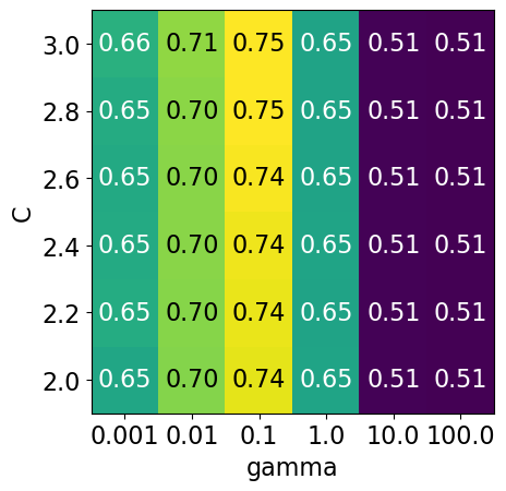
Note that the range we pick for the parameters play an important role in hyperparameter optimization.
For example, consider the following grid and the corresponding results.
param_grid1 = {
"svc__gamma": 10.0**np.arange(-3, 3, 1),
"svc__C": 10.0**np.arange(-3, 3, 1)
}
display_heatmap(param_grid1, pipe_svm, X_train, y_train)
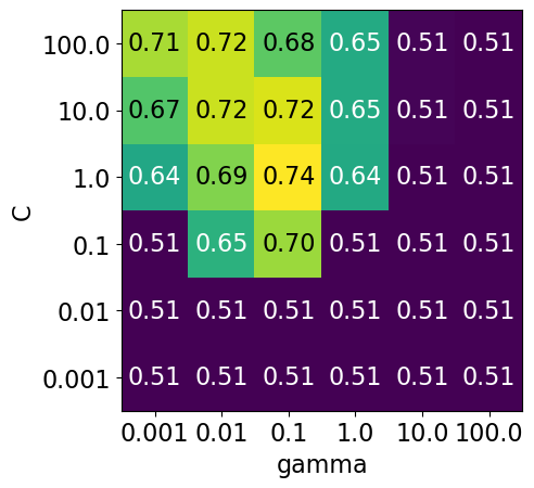
Each point in the heat map corresponds to one run of cross-validation, with a particular setting
Colour encodes cross-validation accuracy.
Lighter colour means high accuracy
Darker colour means low accuracy
SVC is quite sensitive to hyperparameter settings.
Adjusting hyperparameters can change the accuracy from 0.51 to 0.74!
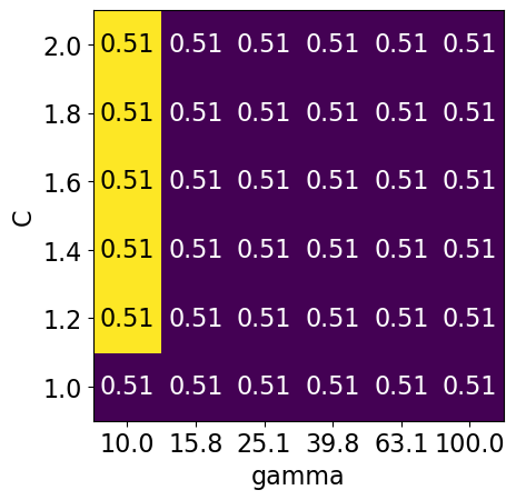
Bad range for hyperparameters#
np.logspace(1, 2, 6)
array([ 10. , 15.84893192, 25.11886432, 39.81071706,
63.09573445, 100. ])
np.linspace(1, 2, 6)
array([1. , 1.2, 1.4, 1.6, 1.8, 2. ])
param_grid2 = {"svc__gamma": np.round(np.logspace(1, 2, 6), 1), "svc__C": np.linspace(1, 2, 6)}
display_heatmap(param_grid2, pipe_svm, X_train, y_train)
Different range for hyperparameters yields better results!#
np.logspace(-3, 2, 6)
array([1.e-03, 1.e-02, 1.e-01, 1.e+00, 1.e+01, 1.e+02])
np.linspace(1, 2, 6)
array([1. , 1.2, 1.4, 1.6, 1.8, 2. ])
param_grid3 = {"svc__gamma": np.logspace(-3, 2, 6), "svc__C": np.linspace(1, 2, 6)}
display_heatmap(param_grid3, pipe_svm, X_train, y_train)
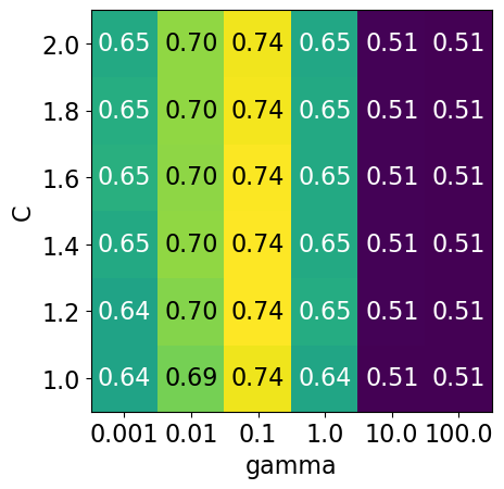
It seems like we are getting even better cross-validation results with C = 2.0 and gamma = 0.1
How about exploring different values of C close to 2.0?
param_grid4 = {"svc__gamma": np.logspace(-3, 2, 6), "svc__C": np.linspace(2, 3, 6)}
display_heatmap(param_grid4, pipe_svm, X_train, y_train)
That’s good! We are finding some more options for C where the accuracy is 0.75.
The tricky part is we do not know in advance what range of hyperparameters might work the best for the given problem, model, and the dataset.
Note
GridSearchCV allows the param_grid to be a list of dictionaries. Sometimes some hyperparameters are applicable only for certain models.
For example, in the context of SVC, C and gamma are applicable when the kernel is rbf whereas only C is applicable for kernel="linear".
Problems with exhaustive grid search#
Required number of models to evaluate grows exponentially with the dimensionally of the configuration space.
Example: Suppose you have
5 hyperparameters
10 different values for each hyperparameter
You’ll be evaluating \(10^5=100,000\) models! That is you’ll be calling
cross_validate100,000 times!
Exhaustive search may become infeasible fairly quickly.
Other options?
Randomized hyperparameter search#
Randomized hyperparameter optimization
Samples configurations at random until certain budget (e.g., time) is exhausted
from sklearn.model_selection import RandomizedSearchCV
param_grid = {
"columntransformer__countvectorizer__max_features": [100, 200, 400, 800, 1000, 2000],
"svc__gamma": [0.001, 0.01, 0.1, 1.0, 10, 100],
"svc__C": np.linspace(2, 3, 6),
}
print("Grid size: %d" % (np.prod(list(map(len, param_grid.values())))))
param_grid
Grid size: 216
{'columntransformer__countvectorizer__max_features': [100,
200,
400,
800,
1000,
2000],
'svc__gamma': [0.001, 0.01, 0.1, 1.0, 10, 100],
'svc__C': array([2. , 2.2, 2.4, 2.6, 2.8, 3. ])}
# Create a random search object
random_search = RandomizedSearchCV(pipe_svm,
param_distributions = param_grid,
n_iter=100,
n_jobs=-1,
return_train_score=True)
# Carry out the search
random_search.fit(X_train, y_train)
RandomizedSearchCV(estimator=Pipeline(steps=[('columntransformer',
ColumnTransformer(transformers=[('standardscaler', StandardScaler(),
                                 ['acousticness', 'danceability', 'energy',
                                  'instrumentalness', 'liveness', 'loudness',
                                  'speechiness', 'tempo', 'valence']),
                                ('onehotencoder',
                                 OneHotEncoder(handle_unknown='ignore'),
                                 ['time_signature', 'key']),
                                ('passthrough', 'passthrough', ['mode']),
                                ('countvectorizer',
                                 CountVectorizer(max_features=100,
                                                 stop_words='english'),
'song_title')])),
('svc', SVC())]),
n_iter=100, n_jobs=-1,
param_distributions={'columntransformer__countvectorizer__max_features': [100,
200,
400,
800,
1000,
2000],
'svc__C': array([2. , 2.2, 2.4, 2.6, 2.8, 3. ]),
'svc__gamma': [0.001, 0.01, 0.1, 1.0,
10, 100]},
return_train_score=True)In a Jupyter environment, please rerun this cell to show the HTML representation or trust the notebook. On GitHub, the HTML representation is unable to render, please try loading this page with nbviewer.org.
RandomizedSearchCV(estimator=Pipeline(steps=[('columntransformer',
                                              ColumnTransformer(transformers=[('standardscaler',
                                                                               StandardScaler(),
                                                                               ['acousticness',
                                                                                'danceability',
                                                                                'energy',
                                                                                'instrumentalness',
                                                                                'liveness',
                                                                                'loudness',
                                                                                'speechiness',
                                                                                'tempo',
                                                                                'valence']),
                                                                              ('onehotencoder',
                                                                               OneHotEncoder(handle_unknown='ignore'),
                                                                               ['time_signature',
                                                                                'key']),
                                                                              ('passthrough',
                                                                               'passthrough',
                                                                               ['mode']),
                                                                              ('countvectorizer',
                                                                               CountVectorizer(max_features=100,
                                                                                               stop_words='english'),
                                                                               'song_title')])),
                                             ('svc', SVC())]),
                   n_iter=100, n_jobs=-1,
                   param_distributions={'columntransformer__countvectorizer__max_features': [100,
                                                                                             200,
                                                                                             400,
                                                                                             800,
                                                                                             1000,
                                                                                             2000],
                                        'svc__C': array([2. , 2.2, 2.4, 2.6, 2.8, 3. ]),
                                        'svc__gamma': [0.001, 0.01, 0.1, 1.0,
                                                       10, 100]},
return_train_score=True)Pipeline(steps=[('columntransformer',
ColumnTransformer(transformers=[('standardscaler', StandardScaler(),
                                 ['acousticness', 'danceability', 'energy',
                                  'instrumentalness', 'liveness', 'loudness',
                                  'speechiness', 'tempo', 'valence']),
                                ('onehotencoder',
                                 OneHotEncoder(handle_unknown='ignore'),
                                 ['time_signature', 'key']),
                                ('passthrough', 'passthrough', ['mode']),
                                ('countvectorizer',
                                 CountVectorizer(max_features=100,
                                                 stop_words='english'),
'song_title')])),
('svc', SVC(C=np.float64(2.8), gamma=0.1))])ColumnTransformer(transformers=[('standardscaler', StandardScaler(),
['acousticness', 'danceability', 'energy',
'instrumentalness', 'liveness', 'loudness',
'speechiness', 'tempo', 'valence']),
('onehotencoder',
OneHotEncoder(handle_unknown='ignore'),
['time_signature', 'key']),
('passthrough', 'passthrough', ['mode']),
('countvectorizer',
CountVectorizer(max_features=100,
stop_words='english'),
'song_title')])['acousticness', 'danceability', 'energy', 'instrumentalness', 'liveness', 'loudness', 'speechiness', 'tempo', 'valence']
StandardScaler()
['time_signature', 'key']
OneHotEncoder(handle_unknown='ignore')
['mode']
passthrough
song_title
CountVectorizer(max_features=100, stop_words='english')
SVC(C=np.float64(2.8), gamma=0.1)
pd.DataFrame(random_search.cv_results_)[
    [
        "mean_test_score",
        "param_columntransformer__countvectorizer__max_features",
        "param_svc__gamma",
        "param_svc__C",
        "mean_fit_time",
        "rank_test_score",
    ]
].set_index("rank_test_score").sort_index().T
| rank_test_score | 1 | 2 | 3 | 4 | 5 | 6 | 7 | 7 | 9 | 10 | ... | 81 | 81 | 81 | 81 | 81 | 81 | 81 | 81 | 81 | 81 |
|---|---|---|---|---|---|---|---|---|---|---|---|---|---|---|---|---|---|---|---|---|---|
| mean_test_score | 0.745801 | 0.745178 | 0.743949 | 0.743324 | 0.743323 | 0.742709 | 0.742088 | 0.742088 | 0.742086 | 0.741465 | ... | 0.508371 | 0.508371 | 0.508371 | 0.508371 | 0.508371 | 0.508371 | 0.508371 | 0.508371 | 0.508371 | 0.508371 |
| param_columntransformer__countvectorizer__max_features | 100.000000 | 100.000000 | 400.000000 | 2000.000000 | 200.000000 | 2000.000000 | 2000.000000 | 400.000000 | 1000.000000 | 400.000000 | ... | 100.000000 | 200.000000 | 400.000000 | 200.000000 | 400.000000 | 200.000000 | 1000.000000 | 100.000000 | 100.000000 | 400.000000 |
| param_svc__gamma | 0.100000 | 0.100000 | 0.100000 | 0.100000 | 0.100000 | 0.100000 | 0.100000 | 0.100000 | 0.100000 | 0.100000 | ... | 100.000000 | 100.000000 | 100.000000 | 100.000000 | 100.000000 | 100.000000 | 100.000000 | 100.000000 | 100.000000 | 100.000000 |
| param_svc__C | 2.800000 | 3.000000 | 2.800000 | 2.200000 | 2.600000 | 2.800000 | 2.600000 | 2.600000 | 2.800000 | 2.400000 | ... | 2.600000 | 2.600000 | 2.600000 | 2.800000 | 2.200000 | 2.400000 | 2.200000 | 3.000000 | 2.200000 | 3.000000 |
| mean_fit_time | 0.064265 | 0.062666 | 0.078317 | 0.094905 | 0.068370 | 0.106957 | 0.103127 | 0.069734 | 0.092470 | 0.070909 | ... | 0.074714 | 0.081843 | 0.083615 | 0.082164 | 0.085600 | 0.076820 | 0.091149 | 0.083562 | 0.085417 | 0.089004 |
5 rows × 100 columns
n_iter#
Note the
n_iter, we didn’t need this forGridSearchCV.Larger
n_iterwill take longer but it’ll do more searching.Remember you still need to multiply by number of folds!
I have set the
random_statefor reproducibility but you don’t have to do it.
Passing probability distributions to random search#
Another thing we can do is give probability distributions to draw from:
from scipy.stats import expon, lognorm, loguniform, randint, uniform, norm, randint
np.random.seed(123)
def plot_distribution(y, bins, dist_name="uniform", x_label='Value', y_label="Frequency"):
    plt.hist(y, bins=bins, edgecolor='blue')
    plt.title('Histogram of values from a {} distribution'.format(dist_name))
    plt.xlabel('Value')
    plt.ylabel('Frequency')
    plt.show()
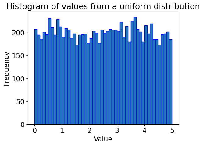
Uniform distribution#
# Generate random values from a uniform distribution
y = uniform.rvs(0, 5, size=10000)

# Creating bins within the range of the data
bins = np.arange(0, 5.1, 0.1)  # Bins from 0 to 5, in increments of 0.1

plot_distribution(y, bins, "uniform")
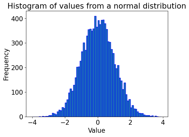
Gaussian distribution#
y = norm.rvs(0, 1, 10000)

# Creating bins
bins = np.arange(-4, 4, 0.1)

plot_distribution(y, bins, "normal")  # Corrected distribution name
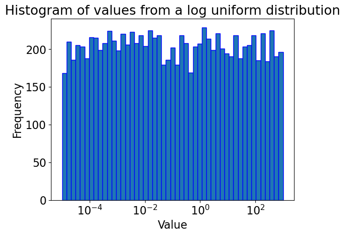
# Generate random values from a log-uniform distribution
# Using loguniform from scipy.stats, specifying a range using the exponents
y = loguniform.rvs(1e-5, 1e3, size=10000)

# Creating bins on a logarithmic scale for better visualization
bins = np.logspace(np.log10(1e-5), np.log10(1e3), 50)
plt.xscale('log')

plot_distribution(y, bins, "log uniform")  # Corrected distribution name
pipe_svm
Pipeline(steps=[('columntransformer',
                 ColumnTransformer(transformers=[('standardscaler',
                                                  StandardScaler(),
                                                  ['acousticness',
                                                   'danceability', 'energy',
                                                   'instrumentalness',
                                                   'liveness', 'loudness',
                                                   'speechiness', 'tempo',
                                                   'valence']),
                                                 ('onehotencoder',
                                                  OneHotEncoder(handle_unknown='ignore'),
                                                  ['time_signature', 'key']),
                                                 ('passthrough', 'passthrough',
                                                  ['mode']),
                                                 ('countvectorizer',
                                                  CountVectorizer(max_features=100,
                                                                  stop_words='english'),
                                                  'song_title')])),
                ('svc', SVC())])
In a Jupyter environment, please rerun this cell to show the HTML representation or trust the notebook. On GitHub, the HTML representation is unable to render, please try loading this page with nbviewer.org.
Pipeline(steps=[('columntransformer',
                 ColumnTransformer(transformers=[('standardscaler',
                                                  StandardScaler(),
                                                  ['acousticness',
                                                   'danceability', 'energy',
                                                   'instrumentalness',
                                                   'liveness', 'loudness',
                                                   'speechiness', 'tempo',
                                                   'valence']),
                                                 ('onehotencoder',
                                                  OneHotEncoder(handle_unknown='ignore'),
                                                  ['time_signature', 'key']),
                                                 ('passthrough', 'passthrough',
                                                  ['mode']),
                                                 ('countvectorizer',
                                                  CountVectorizer(max_features=100,
                                                                  stop_words='english'),
                                                  'song_title')])),
('svc', SVC())])ColumnTransformer(transformers=[('standardscaler', StandardScaler(),
['acousticness', 'danceability', 'energy',
'instrumentalness', 'liveness', 'loudness',
'speechiness', 'tempo', 'valence']),
('onehotencoder',
OneHotEncoder(handle_unknown='ignore'),
['time_signature', 'key']),
('passthrough', 'passthrough', ['mode']),
('countvectorizer',
CountVectorizer(max_features=100,
stop_words='english'),
'song_title')])['acousticness', 'danceability', 'energy', 'instrumentalness', 'liveness', 'loudness', 'speechiness', 'tempo', 'valence']
StandardScaler()
['time_signature', 'key']
OneHotEncoder(handle_unknown='ignore')
['mode']
passthrough
song_title
CountVectorizer(max_features=100, stop_words='english')
SVC()
from scipy.stats import randint

param_dist = {
    "columntransformer__countvectorizer__max_features": randint(100, 2000),
    "svc__C": loguniform(1e-3, 1e3),
    "svc__gamma": loguniform(1e-5, 1e3),
}
# Create a random search object
random_search = RandomizedSearchCV(pipe_svm,
                  param_distributions = param_dist,
                  n_iter=100,
                  n_jobs=-1,
                  return_train_score=True)

# Carry out the search
random_search.fit(X_train, y_train)
RandomizedSearchCV(estimator=Pipeline(steps=[('columntransformer',
                                              ColumnTransformer(transformers=[('standardscaler',
                                                                               StandardScaler(),
                                                                               ['acousticness',
                                                                                'danceability',
                                                                                'energy',
                                                                                'instrumentalness',
                                                                                'liveness',
                                                                                'loudness',
                                                                                'speechiness',
                                                                                'tempo',
                                                                                'valence']),
                                                                              ('onehotencoder',
                                                                               OneHotEncoder(handle_unknown='ignore'),
                                                                               ['time_signature',
                                                                                'key']),
                                                                              ('passthrough',
                                                                               'pass...
                   n_iter=100, n_jobs=-1,
                   param_distributions={'columntransformer__countvectorizer__max_features': <scipy.stats._distn_infrastructure.rv_discrete_frozen object at 0x155a7dbb0>,
                                        'svc__C': <scipy.stats._distn_infrastructure.rv_continuous_frozen object at 0x155a12240>,
                                        'svc__gamma': <scipy.stats._distn_infrastructure.rv_continuous_frozen object at 0x155b55910>},
                   return_train_score=True)
In a Jupyter environment, please rerun this cell to show the HTML representation or trust the notebook. On GitHub, the HTML representation is unable to render, please try loading this page with nbviewer.org.
RandomizedSearchCV(estimator=Pipeline(steps=[('columntransformer',
                                              ColumnTransformer(transformers=[('standardscaler',
                                                                               StandardScaler(),
                                                                               ['acousticness',
                                                                                'danceability',
                                                                                'energy',
                                                                                'instrumentalness',
                                                                                'liveness',
                                                                                'loudness',
                                                                                'speechiness',
                                                                                'tempo',
                                                                                'valence']),
                                                                              ('onehotencoder',
                                                                               OneHotEncoder(handle_unknown='ignore'),
                                                                               ['time_signature',
                                                                                'key']),
                                                                              ('passthrough',
                                                                               'pass...
                   n_iter=100, n_jobs=-1,
                   param_distributions={'columntransformer__countvectorizer__max_features': <scipy.stats._distn_infrastructure.rv_discrete_frozen object at 0x155a7dbb0>,
                                        'svc__C': <scipy.stats._distn_infrastructure.rv_continuous_frozen object at 0x155a12240>,
                                        'svc__gamma': <scipy.stats._distn_infrastructure.rv_continuous_frozen object at 0x155b55910>},
return_train_score=True)Pipeline(steps=[('columntransformer',
ColumnTransformer(transformers=[('standardscaler', StandardScaler(),
                                 ['acousticness', 'danceability', 'energy',
                                  'instrumentalness', 'liveness', 'loudness',
                                  'speechiness', 'tempo', 'valence']),
                                ('onehotencoder',
                                 OneHotEncoder(handle_unknown='ignore'),
                                 ['time_signature', 'key']),
                                ('passthrough', 'passthrough', ['mode']),
                                ('countvectorizer',
                                 CountVectorizer(max_features=1619,
                                                 stop_words='english'),
'song_title')])),
('svc',
SVC(C=np.float64(33.94487839624894),
gamma=np.float64(0.1235387316046016)))])ColumnTransformer(transformers=[('standardscaler', StandardScaler(),
['acousticness', 'danceability', 'energy',
'instrumentalness', 'liveness', 'loudness',
'speechiness', 'tempo', 'valence']),
('onehotencoder',
OneHotEncoder(handle_unknown='ignore'),
['time_signature', 'key']),
('passthrough', 'passthrough', ['mode']),
('countvectorizer',
CountVectorizer(max_features=1619,
stop_words='english'),
'song_title')])['acousticness', 'danceability', 'energy', 'instrumentalness', 'liveness', 'loudness', 'speechiness', 'tempo', 'valence']
StandardScaler()
['time_signature', 'key']
OneHotEncoder(handle_unknown='ignore')
['mode']
passthrough
song_title
CountVectorizer(max_features=1619, stop_words='english')
SVC(C=np.float64(33.94487839624894), gamma=np.float64(0.1235387316046016))
random_search.best_score_
np.float64(0.7278214718381631)
pd.DataFrame(random_search.cv_results_)[
    [
        "mean_test_score",
        "param_columntransformer__countvectorizer__max_features",
        "param_svc__gamma",
        "param_svc__C",
        "mean_fit_time",
        "rank_test_score",
    ]
].set_index("rank_test_score").sort_index().T
| rank_test_score | 1 | 2 | 3 | 4 | 5 | 6 | 7 | 8 | 9 | 10 | ... | 53 | 53 | 53 | 53 | 53 | 53 | 53 | 53 | 99 | 99 |
|---|---|---|---|---|---|---|---|---|---|---|---|---|---|---|---|---|---|---|---|---|---|
| mean_test_score | 0.727821 | 0.727197 | 0.725960 | 0.724722 | 0.722887 | 0.722856 | 0.721616 | 0.721031 | 0.720393 | 0.720383 | ... | 0.507750 | 0.507750 | 0.507750 | 0.507750 | 0.507750 | 0.507750 | 0.507750 | 0.507750 | 0.507130 | 0.507130 |
| param_columntransformer__countvectorizer__max_features | 1619.000000 | 771.000000 | 780.000000 | 694.000000 | 1997.000000 | 830.000000 | 688.000000 | 1738.000000 | 368.000000 | 632.000000 | ... | 958.000000 | 1907.000000 | 322.000000 | 1397.000000 | 1691.000000 | 1606.000000 | 280.000000 | 579.000000 | 1084.000000 | 776.000000 |
| param_svc__gamma | 0.123539 | 0.111841 | 0.011992 | 0.011258 | 0.032324 | 0.012971 | 0.336735 | 0.018201 | 0.007577 | 0.003878 | ... | 0.012152 | 1.902232 | 0.000978 | 0.000361 | 0.000228 | 0.006429 | 0.858475 | 0.000012 | 0.000013 | 268.760262 |
| param_svc__C | 33.944878 | 0.398068 | 12.687613 | 15.748977 | 59.036869 | 32.460294 | 126.368080 | 97.678347 | 6.675570 | 46.455837 | ... | 0.005061 | 0.037578 | 0.001252 | 0.014485 | 0.008073 | 0.001596 | 0.146673 | 0.003795 | 16.705286 | 43.815732 |
| mean_fit_time | 0.109229 | 0.075182 | 0.080986 | 0.074781 | 0.116353 | 0.084855 | 0.097927 | 0.147433 | 0.067821 | 0.070085 | ... | 0.088347 | 0.102500 | 0.073730 | 0.092332 | 0.091821 | 0.093057 | 0.081125 | 0.065103 | 0.081962 | 0.087167 |
5 rows × 100 columns
This is a bit fancy. What’s nice is that you can have it concentrate more on certain values by setting the distribution.
Advantages of RandomizedSearchCV#
Faster compared to
GridSearchCV.Adding parameters that do not influence the performance does not affect efficiency.
Works better when some parameters are more important than others.
In general, I recommend using
RandomizedSearchCVrather thanGridSearchCV.
Advantages of RandomizedSearchCV#
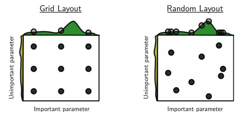
Source: Bergstra and Bengio, Random Search for Hyper-Parameter Optimization, JMLR 2012.
The yellow on the left shows how your scores are going to change when you vary the unimportant hyperparameter.
The green on the top shows how your scores are going to change when you vary the important hyperparameter.
You don’t know in advance which hyperparameters are important for your problem.
In the left figure, 6 of the 9 searches are useless because they are only varying the unimportant parameter.
In the right figure, all 9 searches are useful.
(Optional) Searching for optimal parameters with successive halving¶#
Successive halving is an iterative selection process where all candidates (the parameter combinations) are evaluated with a small amount of resources (e.g., small amount of training data) at the first iteration.
Checkout successive halving with grid search and random search.
from sklearn.experimental import enable_halving_search_cv  # noqa
from sklearn.model_selection import HalvingRandomSearchCV
rsh = HalvingRandomSearchCV(
    estimator=pipe_svm, param_distributions=param_dist, factor=2, random_state=123
)
rsh.fit(X_train, y_train)
HalvingRandomSearchCV(estimator=Pipeline(steps=[('columntransformer',
                                                 ColumnTransformer(transformers=[('standardscaler',
                                                                                  StandardScaler(),
                                                                                  ['acousticness',
                                                                                   'danceability',
                                                                                   'energy',
                                                                                   'instrumentalness',
                                                                                   'liveness',
                                                                                   'loudness',
                                                                                   'speechiness',
                                                                                   'tempo',
                                                                                   'valence']),
                                                                                 ('onehotencoder',
                                                                                  OneHotEncoder(handle_unknown='ignore'),
                                                                                  ['time_signature',
                                                                                   'key']),
                                                                                 ('passthrough',
                                                                                  'p...
                                                ('svc', SVC())]),
                      factor=2,
                      param_distributions={'columntransformer__countvectorizer__max_features': <scipy.stats._distn_infrastructure.rv_discrete_frozen object at 0x155a7dbb0>,
                                           'svc__C': <scipy.stats._distn_infrastructure.rv_continuous_frozen object at 0x155a12240>,
                                           'svc__gamma': <scipy.stats._distn_infrastructure.rv_continuous_frozen object at 0x155b55910>},
                      random_state=123)
In a Jupyter environment, please rerun this cell to show the HTML representation or trust the notebook. On GitHub, the HTML representation is unable to render, please try loading this page with nbviewer.org.
HalvingRandomSearchCV(estimator=Pipeline(steps=[('columntransformer',
                                                 ColumnTransformer(transformers=[('standardscaler',
                                                                                  StandardScaler(),
                                                                                  ['acousticness',
                                                                                   'danceability',
                                                                                   'energy',
                                                                                   'instrumentalness',
                                                                                   'liveness',
                                                                                   'loudness',
                                                                                   'speechiness',
                                                                                   'tempo',
                                                                                   'valence']),
                                                                                 ('onehotencoder',
                                                                                  OneHotEncoder(handle_unknown='ignore'),
                                                                                  ['time_signature',
                                                                                   'key']),
                                                                                 ('passthrough',
                                                                                  'p...
                                                ('svc', SVC())]),
                      factor=2,
                      param_distributions={'columntransformer__countvectorizer__max_features': <scipy.stats._distn_infrastructure.rv_discrete_frozen object at 0x155a7dbb0>,
                                           'svc__C': <scipy.stats._distn_infrastructure.rv_continuous_frozen object at 0x155a12240>,
                                           'svc__gamma': <scipy.stats._distn_infrastructure.rv_continuous_frozen object at 0x155b55910>},
random_state=123)Pipeline(steps=[('columntransformer',
ColumnTransformer(transformers=[('standardscaler', StandardScaler(),
                                 ['acousticness', 'danceability', 'energy',
                                  'instrumentalness', 'liveness', 'loudness',
                                  'speechiness', 'tempo', 'valence']),
                                ('onehotencoder',
                                 OneHotEncoder(handle_unknown='ignore'),
                                 ['time_signature', 'key']),
                                ('passthrough', 'passthrough', ['mode']),
                                ('countvectorizer',
                                 CountVectorizer(max_features=1212,
                                                 stop_words='english'),
'song_title')])),
('svc',
SVC(C=np.float64(2.9601165335428803),
gamma=np.float64(0.1486840817915398)))])ColumnTransformer(transformers=[('standardscaler', StandardScaler(),
['acousticness', 'danceability', 'energy',
'instrumentalness', 'liveness', 'loudness',
'speechiness', 'tempo', 'valence']),
('onehotencoder',
OneHotEncoder(handle_unknown='ignore'),
['time_signature', 'key']),
('passthrough', 'passthrough', ['mode']),
('countvectorizer',
CountVectorizer(max_features=1212,
stop_words='english'),
'song_title')])['acousticness', 'danceability', 'energy', 'instrumentalness', 'liveness', 'loudness', 'speechiness', 'tempo', 'valence']
StandardScaler()
['time_signature', 'key']
OneHotEncoder(handle_unknown='ignore')
['mode']
passthrough
song_title
CountVectorizer(max_features=1212, stop_words='english')
SVC(C=np.float64(2.9601165335428803), gamma=np.float64(0.1486840817915398))
results = pd.DataFrame(rsh.cv_results_)
results["params_str"] = results.params.apply(str)
results.drop_duplicates(subset=("params_str", "iter"), inplace=True)
results
| iter | n_resources | mean_fit_time | std_fit_time | mean_score_time | std_score_time | param_columntransformer__countvectorizer__max_features | param_svc__C | param_svc__gamma | params | ... | std_test_score | rank_test_score | split0_train_score | split1_train_score | split2_train_score | split3_train_score | split4_train_score | mean_train_score | std_train_score | params_str | |
|---|---|---|---|---|---|---|---|---|---|---|---|---|---|---|---|---|---|---|---|---|---|
| 0 | 0 | 20 | 0.004182 | 0.001405 | 0.001950 | 0.000122 | 1634 | 18.955355 | 0.026777 | {'columntransformer__countvectorizer__max_features': 1634, 'svc__C': 18.95535503227586, 'svc__gamma': 0.02677733855112973} | ... | 0.333333 | 110 | 1.000000 | 1.000000 | 1.000000 | 1.000000 | 1.000000 | 1.000000 | 0.000000 | {'columntransformer__countvectorizer__max_features': 1634, 'svc__C': np.float64(18.95535503227586), 'svc__gamma': np.float64(0.02677733855112973)} |
| 1 | 0 | 20 | 0.003163 | 0.000168 | 0.001819 | 0.000140 | 1222 | 2.031836 | 5.698385 | {'columntransformer__countvectorizer__max_features': 1222, 'svc__C': 2.031835829826598, 'svc__gamma': 5.698384608345687} | ... | 0.367423 | 12 | 1.000000 | 1.000000 | 1.000000 | 1.000000 | 1.000000 | 1.000000 | 0.000000 | {'columntransformer__countvectorizer__max_features': 1222, 'svc__C': np.float64(2.031835829826598), 'svc__gamma': np.float64(5.698384608345687)} |
| 2 | 0 | 20 | 0.003119 | 0.000183 | 0.001797 | 0.000139 | 1247 | 47.881370 | 0.019382 | {'columntransformer__countvectorizer__max_features': 1247, 'svc__C': 47.881370370570494, 'svc__gamma': 0.019381838999846482} | ... | 0.333333 | 110 | 1.000000 | 1.000000 | 1.000000 | 1.000000 | 1.000000 | 1.000000 | 0.000000 | {'columntransformer__countvectorizer__max_features': 1247, 'svc__C': np.float64(47.881370370570494), 'svc__gamma': np.float64(0.019381838999846482)} |
| 3 | 0 | 20 | 0.003097 | 0.000224 | 0.001746 | 0.000146 | 213 | 0.768407 | 0.013707 | {'columntransformer__countvectorizer__max_features': 213, 'svc__C': 0.7684071705306555, 'svc__gamma': 0.013706928443177698} | ... | 0.367423 | 12 | 0.666667 | 0.733333 | 0.600000 | 0.812500 | 0.750000 | 0.712500 | 0.072935 | {'columntransformer__countvectorizer__max_features': 213, 'svc__C': np.float64(0.7684071705306555), 'svc__gamma': np.float64(0.013706928443177698)} |
| 4 | 0 | 20 | 0.003060 | 0.000170 | 0.001751 | 0.000153 | 1042 | 5.806335 | 0.003919 | {'columntransformer__countvectorizer__max_features': 1042, 'svc__C': 5.806334557802439, 'svc__gamma': 0.003919287722401839} | ... | 0.367423 | 12 | 0.800000 | 0.733333 | 0.666667 | 0.875000 | 0.750000 | 0.765000 | 0.069602 | {'columntransformer__countvectorizer__max_features': 1042, 'svc__C': np.float64(5.806334557802439), 'svc__gamma': np.float64(0.003919287722401839)} |
| ... | ... | ... | ... | ... | ... | ... | ... | ... | ... | ... | ... | ... | ... | ... | ... | ... | ... | ... | ... | ... | ... |
| 155 | 5 | 640 | 0.010962 | 0.000239 | 0.003481 | 0.000110 | 258 | 1.176468 | 0.051778 | {'columntransformer__countvectorizer__max_features': 258, 'svc__C': 1.1764683596365657, 'svc__gamma': 0.05177790160774991} | ... | 0.050272 | 11 | 0.800391 | 0.812133 | 0.823875 | 0.812500 | 0.820312 | 0.813842 | 0.008101 | {'columntransformer__countvectorizer__max_features': 258, 'svc__C': np.float64(1.1764683596365657), 'svc__gamma': np.float64(0.05177790160774991)} |
| 156 | 5 | 640 | 0.013210 | 0.000180 | 0.003672 | 0.000092 | 440 | 1.546352 | 0.179730 | {'columntransformer__countvectorizer__max_features': 440, 'svc__C': 1.5463515822289584, 'svc__gamma': 0.17973005068132514} | ... | 0.054973 | 8 | 0.980431 | 0.976517 | 0.970646 | 0.988281 | 0.976562 | 0.978487 | 0.005810 | {'columntransformer__countvectorizer__max_features': 440, 'svc__C': np.float64(1.5463515822289584), 'svc__gamma': np.float64(0.17973005068132514)} |
| 157 | 5 | 640 | 0.014759 | 0.000098 | 0.003818 | 0.000114 | 1212 | 2.960117 | 0.148684 | {'columntransformer__countvectorizer__max_features': 1212, 'svc__C': 2.9601165335428803, 'svc__gamma': 0.1486840817915398} | ... | 0.058320 | 7 | 1.000000 | 1.000000 | 1.000000 | 1.000000 | 1.000000 | 1.000000 | 0.000000 | {'columntransformer__countvectorizer__max_features': 1212, 'svc__C': np.float64(2.9601165335428803), 'svc__gamma': np.float64(0.1486840817915398)} |
| 158 | 6 | 1280 | 0.037242 | 0.000579 | 0.007962 | 0.000123 | 440 | 1.546352 | 0.179730 | {'columntransformer__countvectorizer__max_features': 440, 'svc__C': 1.5463515822289584, 'svc__gamma': 0.17973005068132514} | ... | 0.019342 | 6 | 0.959922 | 0.955034 | 0.965787 | 0.968750 | 0.955078 | 0.960914 | 0.005563 | {'columntransformer__countvectorizer__max_features': 440, 'svc__C': np.float64(1.5463515822289584), 'svc__gamma': np.float64(0.17973005068132514)} |
| 159 | 6 | 1280 | 0.045272 | 0.000300 | 0.008975 | 0.000189 | 1212 | 2.960117 | 0.148684 | {'columntransformer__countvectorizer__max_features': 1212, 'svc__C': 2.9601165335428803, 'svc__gamma': 0.1486840817915398} | ... | 0.023031 | 5 | 0.996090 | 0.994135 | 0.995112 | 0.992188 | 0.993164 | 0.994138 | 0.001379 | {'columntransformer__countvectorizer__max_features': 1212, 'svc__C': np.float64(2.9601165335428803), 'svc__gamma': np.float64(0.1486840817915398)} |
160 rows × 26 columns
(Optional) Fancier methods#
Both
GridSearchCVandRandomizedSearchCVdo each trial independently.What if you could learn from your experience, e.g. learn that
max_depth=3is bad?That could save time because you wouldn’t try combinations involving
max_depth=3in the future.
We can do this with
scikit-optimize, which is a completely different package fromscikit-learnIt uses a technique called “model-based optimization” and we’ll specifically use “Bayesian optimization”.
In short, it uses machine learning to predict what hyperparameters will be good.
Machine learning on machine learning!
This is an active research area and there are sophisticated packages for this.
Here are some examples