Lectures 8: Class demo

Imports

import os
import sys

sys.path.append(os.path.join(os.path.abspath(".."), (".."), "code"))
from utils import *
import matplotlib.pyplot as plt
import mglearn
import numpy as np
import pandas as pd
from plotting_functions import *
from sklearn.dummy import DummyClassifier
from sklearn.feature_extraction.text import CountVectorizer, TfidfVectorizer
from sklearn.model_selection import cross_val_score, cross_validate, train_test_split
from sklearn.pipeline import make_pipeline
from sklearn.linear_model import LogisticRegression
%matplotlib inline
pd.set_option("display.max_colwidth", 200)
DATA_DIR = os.path.join(os.path.abspath(".."), (".."), "data/")

Demo: Model interpretation of linear classifiers

• One of the primary advantage of linear classifiers is their ability to interpret models.

• For example, with the sign and magnitude of learned coefficients we could answer questions such as which features are driving the prediction to which direction.

• We’ll demonstrate this by training LogisticRegression on the famous IMDB movie review dataset. The dataset is a bit large for demonstration purposes. So I am going to put a big portion of it in the test split to speed things up.

imdb_df = pd.read_csv(DATA_DIR + "imdb_master.csv", encoding="ISO-8859-1")
imdb_df.head()

	review	sentiment
0	One of the other reviewers has mentioned that after watching just 1 Oz episode you'll be hooked. They are right, as this is exactly what happened with me.<br /><br />The first thing that struck me...	positive
1	A wonderful little production. <br /><br />The filming technique is very unassuming- very old-time-BBC fashion and gives a comforting, and sometimes discomforting, sense of realism to the entire p...	positive
2	I thought this was a wonderful way to spend time on a too hot summer weekend, sitting in the air conditioned theater and watching a light-hearted comedy. The plot is simplistic, but the dialogue i...	positive
3	Basically there's a family where a little boy (Jake) thinks there's a zombie in his closet & his parents are fighting all the time.<br /><br />This movie is slower than a soap opera... and suddenl...	negative
4	Petter Mattei's "Love in the Time of Money" is a visually stunning film to watch. Mr. Mattei offers us a vivid portrait about human relations. This is a movie that seems to be telling us what mone...	positive

Let’s clean up the data a bit.

import re

def replace_tags(doc):
    doc = doc.replace(r"<br />", " ")
    doc = re.sub(r"https://\S*", "", doc)
    return doc

imdb_df["review_pp"] = imdb_df["review"].apply(replace_tags)

Are we breaking the Golden rule here?

Let’s split the data and create bag of words representation.

train_df, test_df = train_test_split(imdb_df, test_size=0.9, random_state=123)
X_train, y_train = train_df["review_pp"], train_df["sentiment"]
X_test, y_test = test_df["review_pp"], test_df["sentiment"]
train_df.shape

(5000, 3)

vec = CountVectorizer(stop_words="english")
bow = vec.fit_transform(X_train)
bow

<Compressed Sparse Row sparse matrix of dtype 'int64'
	with 439384 stored elements and shape (5000, 38867)>

Examining the vocabulary

• The vocabulary (mapping from feature indices to actual words) can be obtained using get_feature_names_out() on the CountVectorizer object.

vocab = vec.get_feature_names_out()

vocab.shape

(38867,)

vocab[0:10]  # first few words

array(['00', '000', '007', '0079', '0080', '0083', '00pm', '00s', '01',
       '0126'], dtype=object)

vocab[2000:2010]  # some middle words

array(['apprehensive', 'apprentice', 'approach', 'approached',
       'approaches', 'approaching', 'appropriate', 'appropriated',
       'appropriately', 'approval'], dtype=object)

vocab[::500]  # words with a step of 500

array(['00', 'aaja', 'affection', 'ambrosine', 'apprehensive', 'attract',
       'barbara', 'bereavement', 'blore', 'brazenly', 'businessman',
       'carrel', 'chatterjee', 'claudio', 'commanding', 'consumed',
       'cramped', 'cynic', 'defining', 'deviates', 'displaced',
       'dramatized', 'edie', 'enforced', 'evolving', 'fanatically',
       'fingertips', 'formal', 'gaffers', 'giogio', 'gravitas',
       'halliday', 'heist', 'hoot', 'iliad', 'infiltrate', 'investment',
       'jobson', 'kidnappee', 'landsbury', 'licentious', 'lousiest',
       'malã', 'maã', 'mice', 'molla', 'museum', 'newtonian',
       'obsessiveness', 'outbursts', 'parapsychologist', 'perpetuates',
       'plasters', 'powers', 'property', 'rabies', 'reclined', 'renters',
       'ridiculous', 'rube', 'sayid', 'select', 'shivers', 'skinheads',
       'sohail', 'spot', 'stomaches', 'suitcase', 'syrupy', 'terrorist',
       'tolerance', 'triangular', 'unbidden', 'unrevealed', 'verneuil',
       'walrus', 'wilcox', 'xxxxviii'], dtype=object)

y_train.value_counts()

sentiment
positive    2517
negative    2483
Name: count, dtype: int64

Model building on the dataset

First let’s try DummyClassifier on the dataset.

dummy = DummyClassifier()
scores = cross_validate(dummy, X_train, y_train, return_train_score=True)
pd.DataFrame(scores)

	fit_time	score_time	test_score	train_score
0	0.001168	0.000660	0.504	0.50325
1	0.000987	0.000596	0.504	0.50325
2	0.000956	0.000570	0.503	0.50350
3	0.000949	0.000566	0.503	0.50350
4	0.000943	0.000564	0.503	0.50350

We have a balanced dataset. So the DummyClassifier score is around 0.5.

Now let’s try logistic regression.

pipe_lr = make_pipeline(
    CountVectorizer(stop_words="english"),
    LogisticRegression(max_iter=1000),
)
scores = cross_validate(pipe_lr, X_train, y_train, return_train_score=True)
pd.DataFrame(scores)

	fit_time	score_time	test_score	train_score
0	0.431325	0.061191	0.828	0.99975
1	0.443467	0.063255	0.830	0.99975
2	0.438494	0.062353	0.848	0.99975
3	0.428711	0.061155	0.833	1.00000
4	0.416827	0.063506	0.840	0.99975

Seems like we are overfitting. Let’s optimize the hyperparameter C of LR and max_features of CountVectorizer.

from scipy.stats import loguniform, randint, uniform
from sklearn.model_selection import RandomizedSearchCV

param_dist = {
    "countvectorizer__max_features": randint(10, len(vocab)),
    "logisticregression__C": loguniform(1e-3, 1e3)
}
pipe_lr = make_pipeline(CountVectorizer(stop_words="english"), LogisticRegression(max_iter=1000))
random_search = RandomizedSearchCV(pipe_lr, param_dist, n_iter=10, n_jobs=-1, return_train_score=True)
random_search.fit(X_train, y_train)

RandomizedSearchCV(estimator=Pipeline(steps=[('countvectorizer',
                                              CountVectorizer(stop_words='english')),
                                             ('logisticregression',
                                              LogisticRegression(max_iter=1000))]),
                   n_jobs=-1,
                   param_distributions={'countvectorizer__max_features': <scipy.stats._distn_infrastructure.rv_discrete_frozen object at 0x17622eed0>,
                                        'logisticregression__C': <scipy.stats._distn_infrastructure.rv_continuous_frozen object at 0x17622ca10>},
                   return_train_score=True)

In a Jupyter environment, please rerun this cell to show the HTML representation or trust the notebook.
On GitHub, the HTML representation is unable to render, please try loading this page with nbviewer.org.

pd.DataFrame(random_search.cv_results_)

	mean_fit_time	std_fit_time	mean_score_time	std_score_time	param_countvectorizer__max_features	param_logisticregression__C	params	split0_test_score	split1_test_score	split2_test_score	...	mean_test_score	std_test_score	rank_test_score	split0_train_score	split1_train_score	split2_train_score	split3_train_score	split4_train_score	mean_train_score	std_train_score
0	0.577830	0.018123	0.109384	0.009253	9931	9.518326	{'countvectorizer__max_features': 9931, 'logisticregression__C': 9.51832640296586}	0.825	0.814	0.835	...	0.8254	0.007864	8	1.00000	1.00000	1.00000	1.00000	1.00000	1.00000	0.000000
1	0.697331	0.092141	0.114220	0.017031	22623	15.748897	{'countvectorizer__max_features': 22623, 'logisticregression__C': 15.748897208303081}	0.826	0.828	0.842	...	0.8322	0.005600	4	1.00000	1.00000	1.00000	1.00000	1.00000	1.00000	0.000000
2	0.686005	0.064007	0.128600	0.008292	36969	0.002231	{'countvectorizer__max_features': 36969, 'logisticregression__C': 0.002231333259815521}	0.816	0.802	0.811	...	0.8120	0.012280	10	0.86375	0.86900	0.86225	0.86300	0.86875	0.86535	0.002918
3	0.585898	0.037224	0.114528	0.010789	19523	0.023044	{'countvectorizer__max_features': 19523, 'logisticregression__C': 0.023043858149902955}	0.843	0.821	0.834	...	0.8370	0.009695	1	0.95300	0.95425	0.95425	0.95325	0.95150	0.95325	0.001012
4	0.579274	0.037246	0.123000	0.028454	36613	171.719120	{'countvectorizer__max_features': 36613, 'logisticregression__C': 171.7191199722997}	0.827	0.828	0.838	...	0.8344	0.005678	2	1.00000	1.00000	1.00000	1.00000	1.00000	1.00000	0.000000
5	0.725929	0.052964	0.121037	0.014576	35524	9.390113	{'countvectorizer__max_features': 35524, 'logisticregression__C': 9.390112899943494}	0.829	0.827	0.843	...	0.8318	0.005741	5	1.00000	1.00000	1.00000	1.00000	1.00000	1.00000	0.000000
6	0.765972	0.105706	0.135371	0.039201	34383	61.666088	{'countvectorizer__max_features': 34383, 'logisticregression__C': 61.666087624102815}	0.821	0.825	0.839	...	0.8318	0.007440	5	1.00000	1.00000	1.00000	1.00000	1.00000	1.00000	0.000000
7	0.798176	0.024560	0.124973	0.020079	15021	216.290450	{'countvectorizer__max_features': 15021, 'logisticregression__C': 216.2904502519345}	0.825	0.826	0.832	...	0.8330	0.007211	3	1.00000	1.00000	1.00000	1.00000	1.00000	1.00000	0.000000
8	0.476637	0.028425	0.105252	0.021404	1242	0.013776	{'countvectorizer__max_features': 1242, 'logisticregression__C': 0.0137760320619256}	0.830	0.803	0.816	...	0.8224	0.013124	9	0.88225	0.88875	0.88100	0.87875	0.88450	0.88305	0.003404
9	0.516189	0.046652	0.103326	0.032167	16201	160.694929	{'countvectorizer__max_features': 16201, 'logisticregression__C': 160.6949292500268}	0.832	0.824	0.829	...	0.8312	0.005564	7	1.00000	1.00000	1.00000	1.00000	1.00000	1.00000	0.000000

10 rows × 22 columns

cv_scores = random_search.cv_results_['mean_test_score']
train_scores = random_search.cv_results_['mean_train_score']
countvec_max_features = random_search.cv_results_['param_countvectorizer__max_features']

pd.DataFrame(random_search.cv_results_)[
    [
        "mean_test_score",
        "mean_train_score",        
        "param_logisticregression__C",
        "param_countvectorizer__max_features",
        "mean_fit_time",
        "rank_test_score",
    ]
].set_index("rank_test_score").sort_index()

	mean_test_score	mean_train_score	param_logisticregression__C	param_countvectorizer__max_features	mean_fit_time
rank_test_score
1	0.8370	0.95325	0.023044	19523	0.585898
2	0.8344	1.00000	171.719120	36613	0.579274
3	0.8330	1.00000	216.290450	15021	0.798176
4	0.8322	1.00000	15.748897	22623	0.697331
5	0.8318	1.00000	9.390113	35524	0.725929
5	0.8318	1.00000	61.666088	34383	0.765972
7	0.8312	1.00000	160.694929	16201	0.516189
8	0.8254	1.00000	9.518326	9931	0.577830
9	0.8224	0.88305	0.013776	1242	0.476637
10	0.8120	0.86535	0.002231	36969	0.686005

Let’s train a model on the full training set with the optimized hyperparameter values.

best_model = random_search.best_estimator_

best_model

Pipeline(steps=[('countvectorizer',
                 CountVectorizer(max_features=19523, stop_words='english')),
                ('logisticregression',
                 LogisticRegression(C=np.float64(0.023043858149902955),
                                    max_iter=1000))])

In a Jupyter environment, please rerun this cell to show the HTML representation or trust the notebook.
On GitHub, the HTML representation is unable to render, please try loading this page with nbviewer.org.

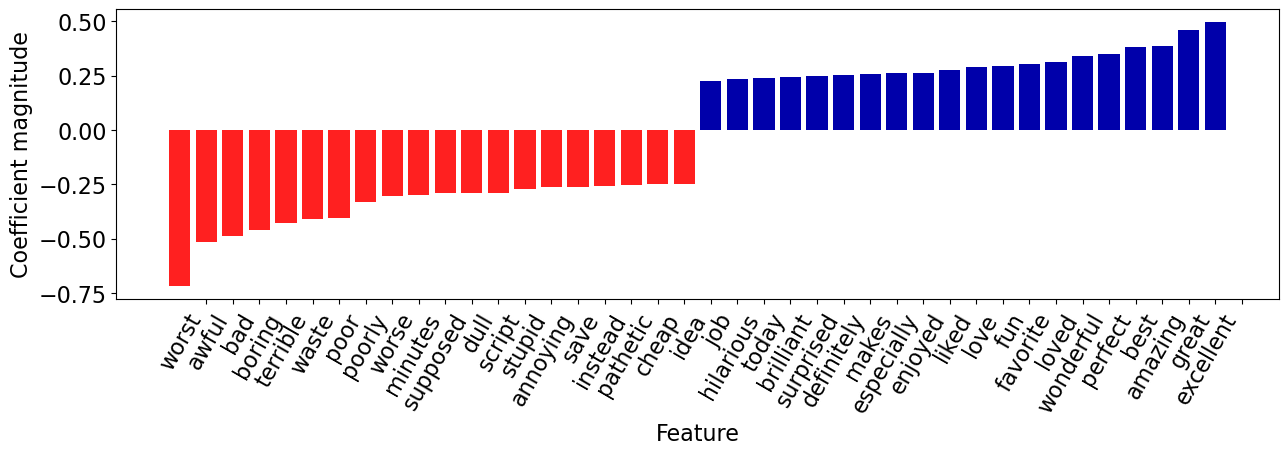
Examining learned coefficients

• The learned coefficients are exposed by the coef_ attribute of LogisticRegression object.

# Get feature names
feature_names = best_model.named_steps['countvectorizer'].get_feature_names_out().tolist()

# Get coefficients 
coeffs = best_model.named_steps["logisticregression"].coef_.flatten()

word_coeff_df = pd.DataFrame(coeffs, index=feature_names, columns=["Coefficient"])
word_coeff_df

	Coefficient
00	0.021804
000	0.021389
007	-0.001506
02	-0.010779
10	0.149399
...	...
zorro	0.017694
zu	0.037692
zucco	-0.029374
zucker	0.014023
â½	-0.004357

19523 rows × 1 columns

• Let’s sort the coefficients in descending order.

• Interpretation

  • if \(w_j > 0\) then increasing \(x_{ij}\) moves us toward predicting \(+1\).

  • if \(w_j < 0\) then increasing \(x_{ij}\) moves us toward predicting \(-1\).

word_coeff_df.sort_values(by="Coefficient", ascending=False)

	Coefficient
excellent	0.495360
great	0.460475
amazing	0.386294
best	0.382126
perfect	0.351134
...	...
terrible	-0.429293
boring	-0.460820
bad	-0.486894
awful	-0.517039
worst	-0.718337

19523 rows × 1 columns

• The coefficients make sense!

Let’s visualize the top 20 features.

mglearn.tools.visualize_coefficients(coeffs, feature_names, n_top_features=20)

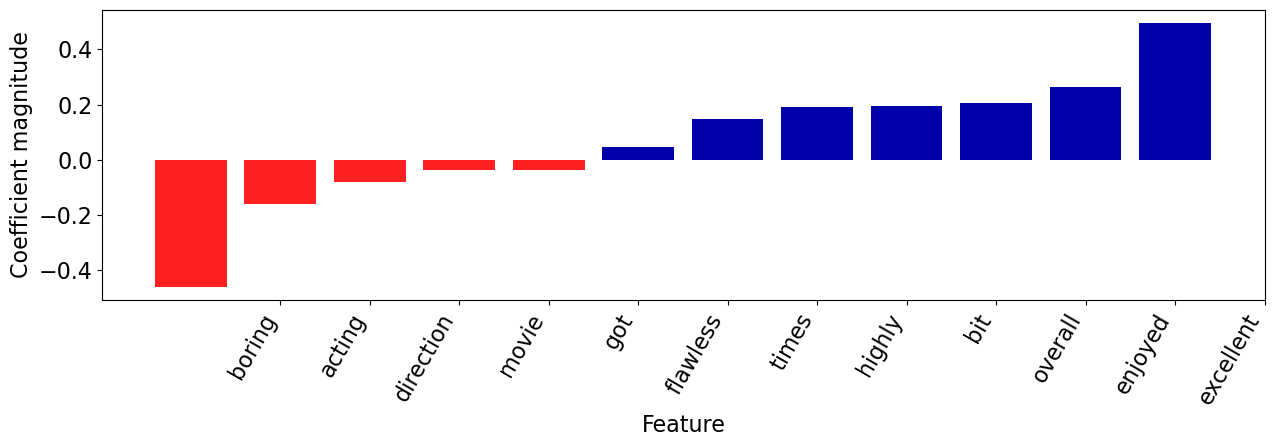
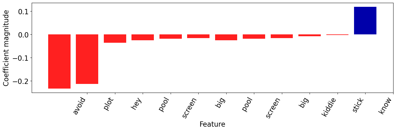
Let’s explore prediction of the following new review.

fake_reviews = ["It got a bit boring at times but the direction was excellent and the acting was flawless. Overall I enjoyed the movie and I highly recommend it!",
 "The plot was shallower than a kiddie pool in a drought, but hey, at least we now know emojis should stick to texting and avoid the big screen."
]

Let’s get prediction probability scores of the fake review.

best_model.predict(fake_reviews)

array(['positive', 'negative'], dtype=object)

# Get prediction probabilities for fake reviews 
best_model.predict_proba(fake_reviews)

array([[0.29130377, 0.70869623],
       [0.60542235, 0.39457765]])

best_model.classes_

array(['negative', 'positive'], dtype=object)

We can find which of the vocabulary words are present in this review:

def plot_coeff_example(model, review, coeffs, feature_names, n_top_feats=6):
    print(review)
    feat_vec = model.named_steps["countvectorizer"].transform([review])
    words_in_ex = feat_vec.toarray().ravel().astype(bool)

    ex_df = pd.DataFrame(
        data=coeffs[words_in_ex],
        index=np.array(feature_names)[words_in_ex],
        columns=["Coefficient"],
    )
    mglearn.tools.visualize_coefficients(
    coeffs[words_in_ex], np.array(feature_names)[words_in_ex], n_top_features=n_top_feats
    )
    return ex_df.sort_values(by=["Coefficient"], ascending=False)

plot_coeff_example(best_model, fake_reviews[0], coeffs, feature_names)

It got a bit boring at times but the direction was excellent and the acting was flawless. Overall I enjoyed the movie and I highly recommend it!

	Coefficient
excellent	0.495360
enjoyed	0.263004
overall	0.205418
bit	0.196344
highly	0.191171
times	0.147928
recommend	0.112222
flawless	0.045797
got	-0.036158
movie	-0.037063
direction	-0.082195
acting	-0.161708
boring	-0.460820

plot_coeff_example(best_model, fake_reviews[1], coeffs, feature_names)

The plot was shallower than a kiddie pool in a drought, but hey, at least we now know emojis should stick to texting and avoid the big screen.

	Coefficient
know	0.117809
stick	-0.002270
kiddie	-0.008865
big	-0.016856
screen	-0.019274
pool	-0.025352
hey	-0.036117
plot	-0.213434
avoid	-0.233514

Most positive review

• Remember that you can look at the probabilities (confidence) of the classifier’s prediction using the model.predict_proba method.

• Can we find the reviews where our classifier is most certain or least certain?

# only get probabilities associated with pos class
pos_probs = best_model.predict_proba(X_train)[
    :, 1
]  # only get probabilities associated with pos class
pos_probs

array([0.94012045, 0.39287447, 0.82836255, ..., 0.63796708, 0.78840048,
       0.04441458])

What’s the index of the example where the classifier is most certain (highest predict_proba score for positive)?

most_positive_id = np.argmax(pos_probs)

print("True target: %s\n" % (y_train.iloc[most_positive_id]))
print("Predicted target: %s\n" % (best_model.predict(X_train.iloc[[most_positive_id]])[0]))
print("Prediction probability: %0.4f" % (pos_probs[most_positive_id]))

True target: positive

Predicted target: positive

Prediction probability: 1.0000

Let’s examine the features associated with the review.

plot_coeff_example(best_model, X_train.iloc[most_positive_id], coeffs, feature_names)

This is an awesome Amicus horror anthology, with 3 great stories, and fantastic performances!, only the last story disappoints. All the characters are awesome, and the film is quite chilling and suspenseful, plus Peter Cushing and Christopher Lee are simply amazing in this!. It's very underrated and my favorite story has to be the 3rd one "Sweets To The Sweet", plus all the characters are very likable. Some of it's predictable, and the last story was incredibly disappointing and rather bland!, however the ending was really cool!. This is an awesome Amicus horror anthology, with 3 great stories, and fantastic performances, only the last story disappoints!, i say it's must see!.  1st Story ("Method for Murder"). This is an awesome story, with plenty of suspense, and the killer Dominic is really creepy, and it's very well acted as well!. This was the perfect way to start off with a story, and for the most part it's unpredictable, plus the double twist ending is shocking, and quite creepy!. Grade A  2nd Story. ("Waxworks"). This is a solid story all around, with wonderful performances, however the ending is quite predictable, but it's still creepy, and has quite a bit of suspense, Peter Cushing did an amazing job, and i couldn't believe how young Joss Ackland was, i really enjoyed this story!. Grade B  3rd Story ("Sweets to the Sweet"). This is the Best story here, as it's extremely creepy, and unpredictable throughout, it also has a nice twist as well!. Christopher Lee did an amazing job, and Chloe Franks did a wonderful job as the young daughter, plus the ending is quite shocking!. I don't want to spoil it for you, but it's one of the best horror stories i have seen!. Grade A+  4th Story ("The Cloak"). This is a terrible story that's really weak and unfunny Jon Pertwee annoyed me, however the ending surprised me a little bit, and Ingrid Pitt was great as always, however it's just dull, and has been done before many times, plus where was the creativity??. Grade D  The Direction is great!. Peter Duffell does a great job here, with awesome camera work, great angles, adding some creepy atmosphere, and keeping the film at a very fast pace!.  The Acting is awesome!. John Bryans is great here, as the narrator, he had some great lines, i just wished he had more screen time. John Bennett is very good as the Det., and was quite intense, he was especially good at the end!, i liked him lots. Denholm Elliott is excellent as Charles, he was vulnerable, showed fear, was very likable, and i loved his facial expressions, he rocked!. Joanna Dunham is stunningly gorgeous!, and did great with what she had to do as the wife, she also had great chemistry with Denholm Elliott !. Tom Adams is incredibly creepy as Dominic, he was creepy looking, and got the job done extremely well!. Peter Cushing is amazing as always, and is amazing here, he is likable, focused, charming, and as always, had a ton of class! (Cushing Rules!!). Joss Ackland is fantastic as always, and looked so young here, i barely recognized him, his accent wasn't so thick, and played a different role i loved it! (Ackland rules). Wolfe Morris is creepy here, and did what he had to do well.Christopher Lee is amazing as always and is amazing here, he is incredibly intense, very focused, and as always had that great intense look on his face, he was especially amazing at the end! (Lee Rules!!). Chloe Franks is adorable as the daughter, she is somewhat creepy, and gave one of the best child performances i have ever seen!, i loved her.Nyree Dawn Porter is beautiful and was excellent as the babysitter, i liked her lots!. Jon Pertwee annoyed me here, and was quite bland, and completely unfunny, he also had no chemistry with Ingrid Pitt!. Ingrid Pitt is beautiful , and does her usual Vampire thing and does it well!.   Rest of the cast do fine. Overall a must see!. **** out of 5

	Coefficient
excellent	0.495360
great	0.460475
amazing	0.386294
best	0.382126
perfect	0.351134
...	...
disappointing	-0.184624
predictable	-0.195405
couldn	-0.245557
dull	-0.288601
terrible	-0.429293

171 rows × 1 columns

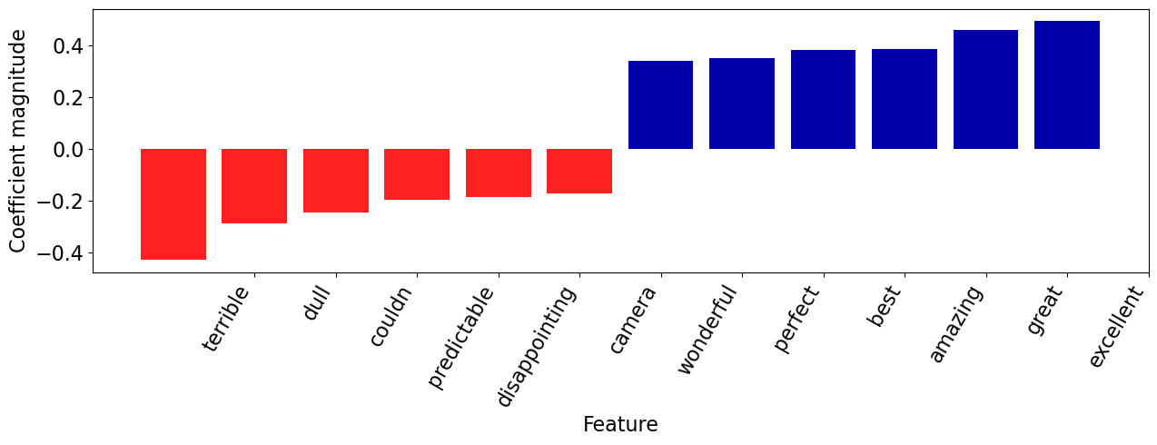
The review has both positive and negative words but the words with positive coefficients win in this case!

Most negative review

neg_probs = best_model.predict_proba(X_train)[
    :, 0
]  # only get probabilities associated with neg class
neg_probs

array([0.05987955, 0.60712553, 0.17163745, ..., 0.36203292, 0.21159952,
       0.95558542])

most_negative_id = np.argmax(neg_probs)

print("Review: %s\n" % (X_train.iloc[[most_negative_id]]))
print("True target: %s\n" % (y_train.iloc[most_negative_id]))
print("Predicted target: %s\n" % (best_model.predict(X_train.iloc[[most_negative_id]])[0]))
print("Prediction probability: %0.4f" % (neg_probs[most_negative_id]))

Review: 13452    Zombi 3 starts as a group of heavily armed men steal a experimental chemical developed to reanimate the dead, while trying to escape the man is shot at & the metal container holding the chemical i...
Name: review_pp, dtype: object

True target: negative

Predicted target: negative

Prediction probability: 1.0000

plot_coeff_example(best_model, X_train.iloc[most_negative_id], coeffs, feature_names)

Zombi 3 starts as a group of heavily armed men steal a experimental chemical developed to reanimate the dead, while trying to escape the man is shot at & the metal container holding the chemical is breached. The man gets some of the green chemical on a wound on his hand which soon after turns him into a flesh eating cannibalistic zombie. Within hours the surrounding area is crawling with the flesh easting undead on the look out for fresh victims, Kenny (Deran Sarafian) & his army buddies find themselves in big trouble as they stop to help Patricia (Beatrice Ring) & her friend Lia (Deborah Bergammi) who has been pecked by zombie birds (!). General Morton is in charge of the situation & has to stop the zombie plague from spread throughout the whole world! But will he & his men succeed?  This Italian produced film was to be directed by Italian zombie gore film auteur Lucio Fulci but the story goes he suffered a stroke & therefore couldn't finish the film so producer Franco Gaudenzi asked second unit director Bruno Mattei & writer Claudio Fragasso to step in & complete the film. Apparently Mattei & Fragasso did more than just finish it they actually disregarded a lot of the footage Fulci shot & added a lot of their own & Zombi 3 ended up as nearly a straight 50/50 split. The script by Fragasso is an absolute mess, none of it is well thought out & is just as stupid as it gets. The scenes of zombie birds attacking people are not only technically inept but the whole idea is just absurd. The zombies themselves have no consistency whatsoever, look at the scene where Patricia is on the bridge & the zombies are slow as they shuffle along but then look at the scene earlier on where she was attacked by the zombie with the machete because that one runs around like it's on steroids, then for no reasonable explanation about 10 minutes before the film finishes the zombies suddenly develop the ability to speak which also looks daft. There are so many things wrong with Zombi 3, scene after scene of terribly thought out & ineptly directed action, awful character's & really dull broken English dialogue which doesn't make sense half the time. Then there's the embarrassing scene where the zombie head inside the fridge suddenly develops the ability to fly through the air & bite someones neck, the scene when the guy's in white contamination suits at the end are about to kill Kenny & Roger but instead of using their automatic rifles they decide to try & kill them by hand, even when Kenny picks up a gun himself they still refuse to use their rifles & when Kenny starts to shoot them all they still refuse to use their rifles & it's one of the most ineptly handled scenes ever put to film & then there's the end where Kenny takes off in the helicopter but can't rest it down on the ground for literally a few seconds to pick his buddy up & then a load of zombies suddenly spring up from under some piles of grass, what? Since when did zombies hide themselves yet alone under piles of grass? This all may sound 'fun' but believe me it's not, it's a really bad film that is just boring, repetitive & simply doesn't work on any level as a piece of entertainment except for a few unintentional laughs.  It's hard to know who was responsible for what exactly but none of the footage is particularly well shot. It has a bland lifeless feel about it & for some reason the makers have tried to bath every scene in mist, the problem is they clearly only had one fog machine & you can see that at one corner of the screen the mist is noticeably thicker as it is coming straight out of the machine & thinning out as it disperses across the scene. Since a lot of it is set during the day it doesn't add any sort of atmosphere whatsoever & when they do get it right & the mist is evenly spread across the screen it just looks like they shot the scene on a foggy day! The direction is poor with no consistency & it just looks & feels bottom of the barrel stuff. Even the blood & gore isn't up to much, there's a gory hand severing at the start, a scene when something rips out of a pregnant woman's stomach, a legless woman (what actually took her legs off in the pool by the way & why didn't it take the legs off the guy who jumped in to save her?) & a few OK looking zombies is as gory as it gets. For anyone hoping to see a gore fest the likes of which Fulci regularly served up during the late 70's & early 80's will be very disappointed, there aren't any decent feeding scenes, no intestines, no stand out 'head shots' & very little gore at all.  Technically the film is poor, the special effects are cheap looking, the cinematography is dull, the music is terrible, the locations are bland & it has rock bottom production values. This was actually shot in the Philippines to keep the cost down to a minimum. The entire film is obviously dubbed, the acting still looks awful though & the English version seems to have been written by someone who doesn't understand the language that well.  Zombi 3 is not a sequel to Fulci's classic zombie gore fest Zombi 2 (1979), it has nothing to do with it at all apart from the cash-in title. I'm sorry but Zombi 3 is an amateurish mess of a film, it's boring, it makes no sense, it's not funny enough to be entertaining & it lacks any decent gore. One to avoid.

	Coefficient
fun	0.293438
makes	0.259262
entertaining	0.181149
10	0.149399
man	0.146621
...	...
poor	-0.407244
terrible	-0.429293
boring	-0.460820
bad	-0.486894
awful	-0.517039

307 rows × 1 columns

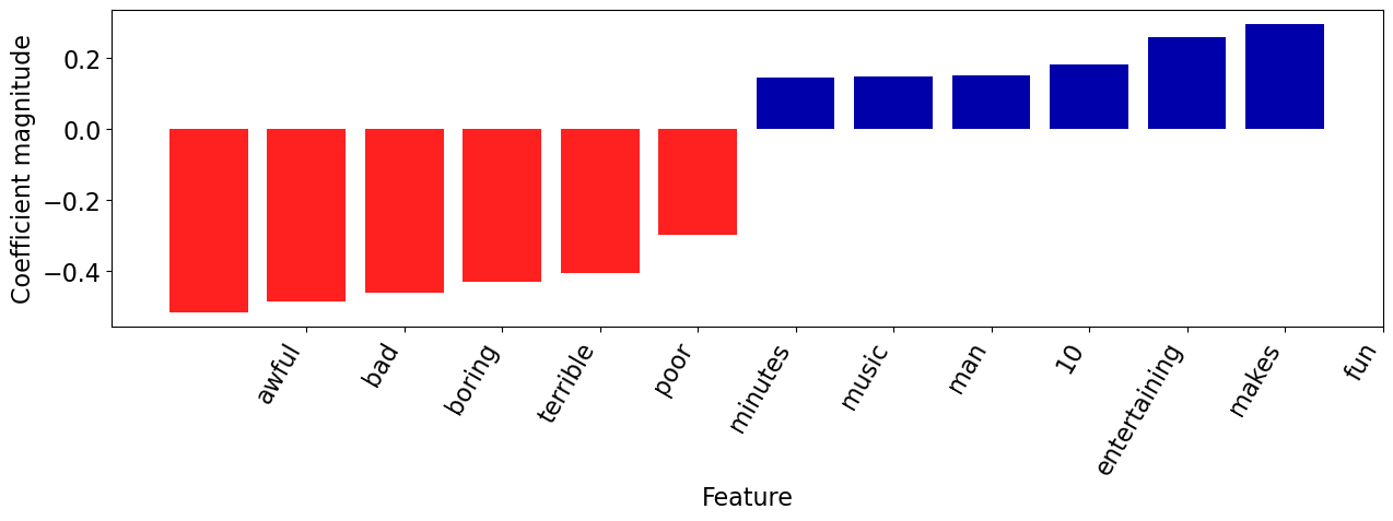
The review has both positive and negative words but the words with negative coefficients win in this case!

❓❓ Questions for you

Question for you to ponder on

• Is it possible to identify most important features using \(k\)-NNs? What about decision trees?