
Lecture 1: Markov Models#
UBC Master of Data Science program, 2024-25
Imports and LO#
Imports#
import os
import re
import sys
import time
from collections import Counter, defaultdict

import IPython
import nltk
import numpy as np
import pandas as pd
from IPython.display import HTML, display
from nltk.corpus import stopwords
from nltk.tokenize import sent_tokenize, word_tokenize
Learning outcomes#
From this lesson you will be able to
Explain the general idea of a language model and name some of its applications.
Define Markov chains and explain terminology (states, initial probability distribution over states, and transition matrix) related to Markov chains.
State Markov assumption.
Compute the probability of a sequence of states.
Compute the probability of being in a state at time \(t\).
Explain the general idea of a stationary distribution.
1. Language models: motivation#
1.1 What is a language model?#
🧠 Activity#
Let’s play a quick game. I’ll give you a phrase, for example:
too much
Now, I want you to guess what word might come next. You can suggest multiple options and even assign rough probabilities to each one.
Next word |
probability |
|---|---|
work |
0.10 |
butter |
0.3 |
rain |
Great! What you just did is what a language model does. It assigns probabilities to possible next words.
We just guessed those numbers based on our intuition. But out in the real world, we’re surrounded by massive amounts of text such as books, websites, social media, and more.
We can use that real data to compute actual probability distributions. For example:
More formally, a language model computes the probability distribution over sequences of tokens or subtokens. Given some vocabulary \(V\), a language model assigns a probability (a number between 0 and 1) to all sequences of tokens or subtokens in \(V\).
Intuitively, this probability tells us how “good” or plausible a sequence of tokens is.
For example:
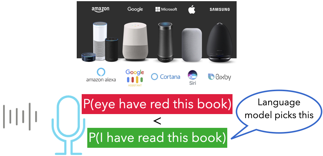
P(I have read this book) > P(eye have red this book) or P(book | read this) > P(book | red this)
P(How do I start a savings habit?) > P(How to start shaving a rabbit?)
One of the most common applications for predicting the next word is the ‘smart compose’ feature in your emails, text messages, and search engines.
url = "https://2.bp.blogspot.com/-KlBuhzV_oFw/WvxP_OAkJ1I/AAAAAAAACu0/T0F6lFZl-2QpS0O7VBMhf8wkUPvnRaPIACLcBGAs/s1600/image2.gif"

IPython.display.IFrame(url, width=500, height=500)
1.2 Language modeling: Why should we care?#
Powerful idea in NLP and helps in many tasks.
From simple Markov models to advanced systems like ChatGPT, all language models are doing this at their core – computing probability distributions over words or tokens or subtokens to predict what comes next.
In old days language models were used as a component of a larger system.
Machine translation
P(In the age of data algorithms have the answer) > P(the age data of in algorithms answer the have)
Spelling correction
My office is a 10 minuet bike ride from my home.
P(10 minute bike ride from my home) > P(10 minuet bike ride from my home)
Speech recognition
P(I read a book) > P(Eye red a book)
Now they are capable of being a standalone systems (e.g., ChatGPT)
Question answering (e.g., Andrei Markov was born in __)
Content generation (e.g., Generating news articles)
Summarization
Writing assistants (e.g., https://www.ai21.com/)
…
Why is this hard?
Language modeling requires not only linguistic expertise but also extensive world knowledge.
The machine learning models we’ve studied so far may not be directly suitable because language modeling demands sequence modeling capabilities.
In this course, we will explore models specifically designed to model sequences effectively.
We’ll start with the simplest kind of language model: the Markov model of language.
Later in the course, we will talk about neural language models.
Today’s lecture will delve into the theory behind Markov models. Our next lecture will examine some real-world applications of Markov models.
Markov chains you have seen in MDS so far
DSCI 512
You wrote code to generate text using Markov models of language.
DSCI 553
You used it as a simulation tool to approximate the posterior distribution of your Bayesian modeling parameters of interest.
The model we are going to look at is similar to what you’ve seen in DSCI 512.
2. Markov model intuition#
2.1 Examples of Markov chains#
🧠 Activity
Each of you will receive a sticky note with a word on it. Here’s what you’ll do:
Carefully remove the sticky note to see the word. This word is for your eyes only; don’t show it to your neighbours!
Think quickly: what word would logically follow the word on the sticky note? Write this next word on a new sticky note. You have about 20 seconds for this step, so trust your instincts!
Pass your predicted word to the person next to you. Do not pass the word you received from your neighbour forward. Keep the chain going!
Stop after the last person in your row/table has finished.
Whichever row generates the most captivating sentence will be rewarded with treats! 🍫
You’ve just created a simple Markov model of language!
In predicting the next word from a minimal context, you likely used your linguistic intuition and familiarity with common two-word phrases or collocations.
You could create more coherent sentences by taking into account more context e.g., previous two words or four words or 100 words.
This idea was first used by Shannon in The Shannon’s game. See this video by Jordan Boyd-Graber for more information on this.
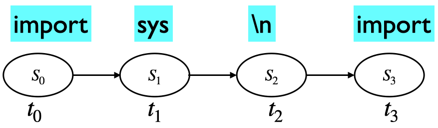
Example: Does this look like Python code?
import sys
import warnings
import ast
import numpy.core.overrides import set_module
# While not in __all__, matrix_power used to be defined here, so we import
# it for backward compatibility
    getT = T.fget
    getI = I.fget
def _from_string(data):
    for char in '[]':
        data = data.replace(char, '')
    rows = str.split(';')
    rowtup = []
        for row in rows:
        trow = newrow
        coltup.append(thismat)
        rowtup.append(concatenate(coltup, axis=-1))
            return NotImplemented
How is this text generated?#
Imagine you have a peculiar kind of memory, like a strange form of amnesia.
You can only remember one word at a time: the current word.
Now picture writing a Python program with this limitation. After writing a word, you forget everything that came before. Your next word choice depends only on the one you just wrote.
To decide what comes next, you consult a list, built from a large collection of Python code, that tells you which words are most likely to follow the current one.
You repeat this step for each word, gradually generating a new sequence.
This is how a Markov model works: it generates text one word at a time, using only the previous word.
You can think of each word as a state, and at each time step, you transition from one state to another based on learned probabilities.
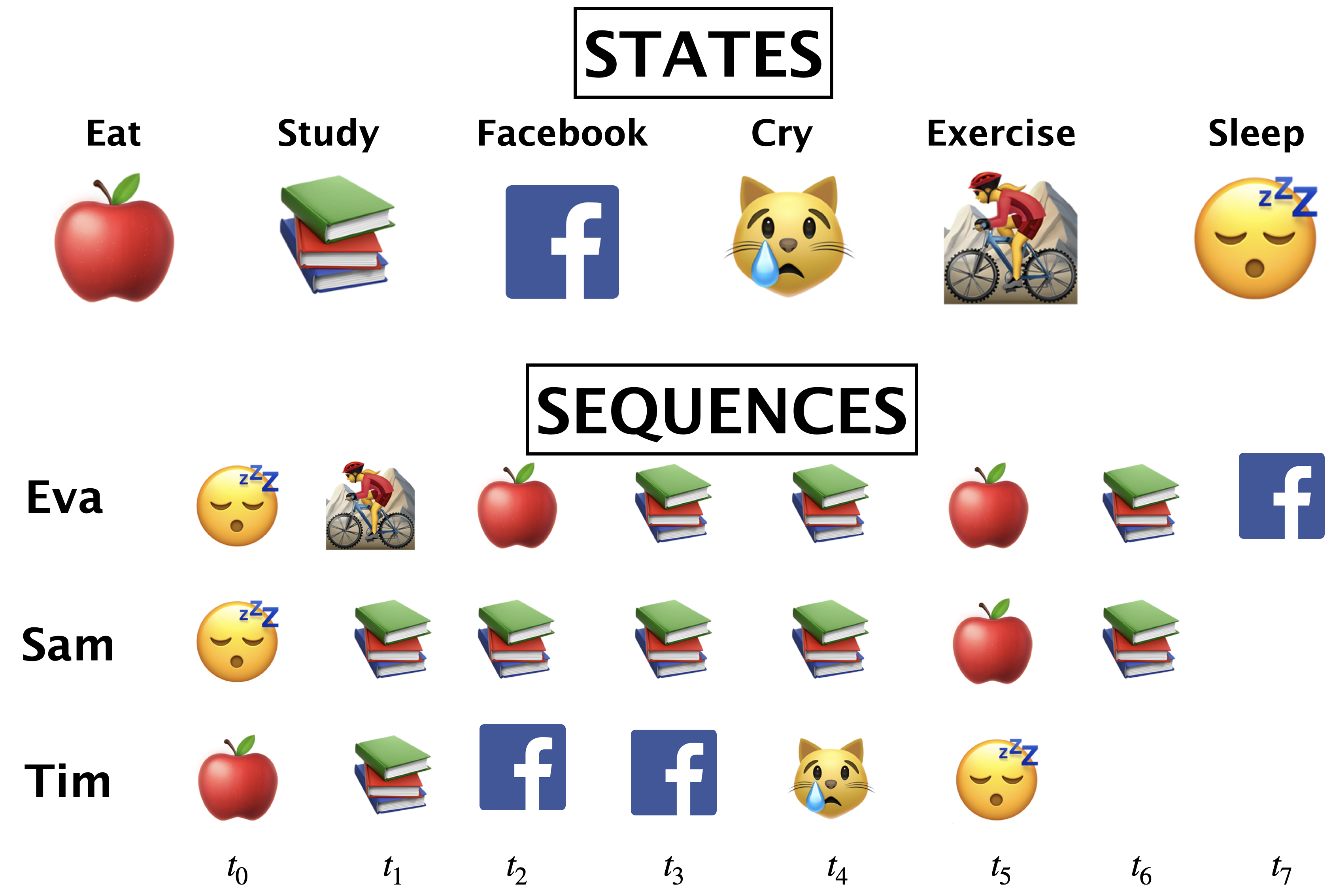
Example with daily activities as states
What kinds of activities does a typical MDS student carry out on a daily basis?
2.2 Markov chain idea#
Often we need to model systems or processes that evolve over time.
We want to represent the state of the world at each specific point via a series of snapshots.
Markov chain idea: Predict future depending upon
the current state
the probability of change
Examples:
Weather: Given that today is cold, what will be the weather tomorrow?
Stock prices: Given the current market conditions what will be the stock prices tomorrow?
Text: Given that the speaker has uttered the word data what will be the next word?
2.3 Markov assumption#
Suppose we want to calculate probability of a sequence “there is a crack in everything that ‘s how the light gets in” (a phrase from Leonard Cohen’s poem Anthem). A naive approach to calculate this probability would be:
You can also express it as a product of conditional probabilities. $\(P(w_{1:n}) = \prod_{i=1}^n P(\text{word}_i \mid \text{word}_{1:i-1})\)$
But this doesn’t take us too far, as calculating probability of a word given the entire history (e.g., \(P(\text{light} \mid \text{there is a crack in everything that 's how the})\)) is not easy because language is creative and any particular context might not have occurred before.
The intuition of Markov models of language (ngram models) is that instead of computing the probability of the next word given its entire history we approximate it by considering just the last few words.
Markov assumption: The future is conditionally independent of the past given present
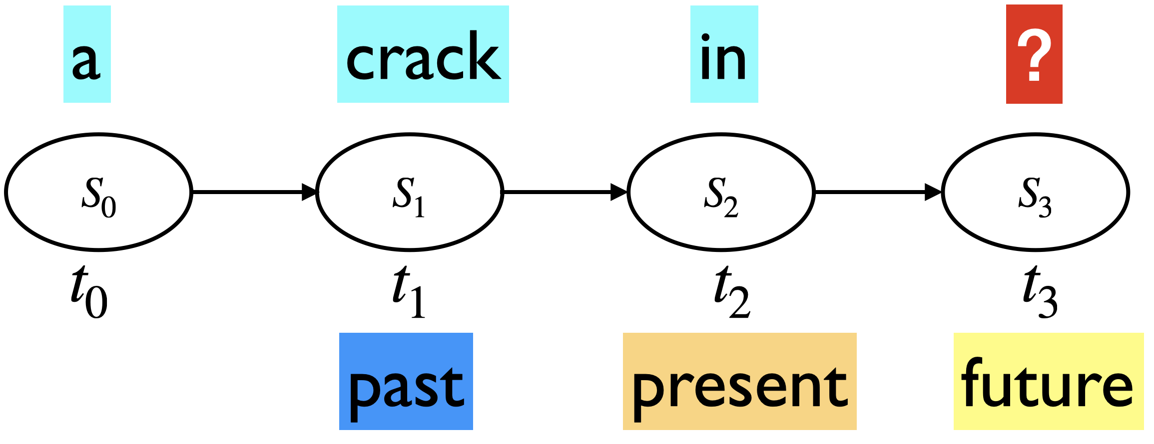
Markov assumption: The future is conditionally independent of the past given present
In the example above
Generalizing it to \(t\) time steps
With Markov’s assumption, the probability of the following sequence would be easier to calculate:
Simplistic auto-complete
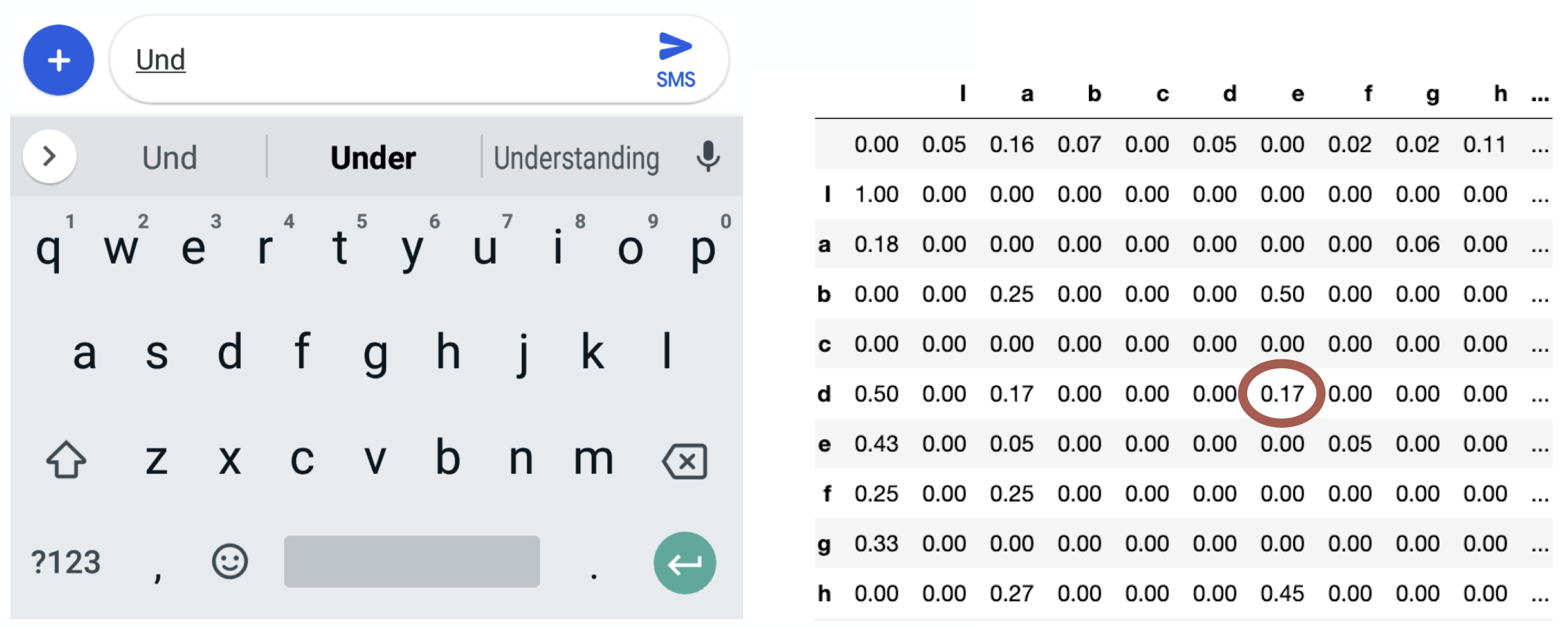
Supposed we have typed “und” so far and we want to predict the next letter, i.e., the state we would be in in the next time step.
Imagine that you have access to the conditional probability distribution for the next letter given the current letter.
We sample the next letter from this distribution.
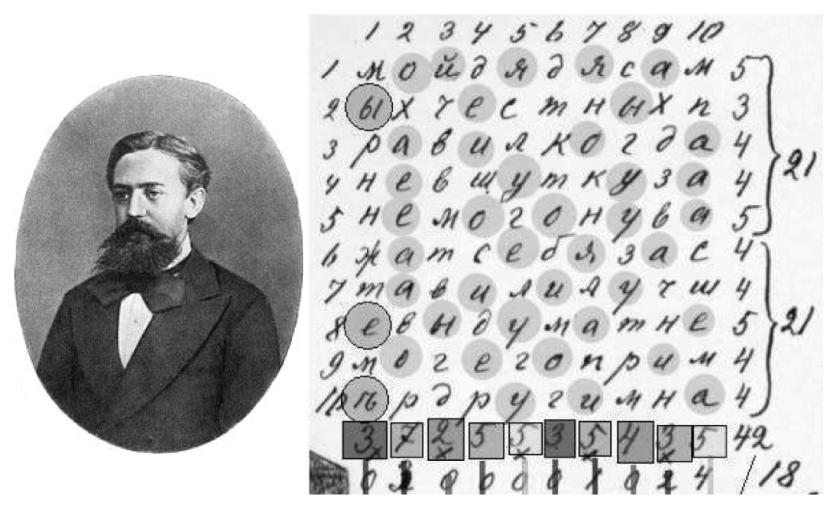
2.4 (ASIDE) Markov’s own application of his chains (1913)#
Studied the sequence of 20,000 letters in A. S. Pushkin’s poem Eugeny Onegin.
Markov also studied the sequence of 100,000 letters in S. T. Aksakov’s novel “The Childhood of Bagrov, the Grandson”.
❓❓ Question for you#
Exercise 1.1 Conditioning and marginalization (revision)#
We will be using the following concepts from probability a lot. So let’s revise them.
Conditioning
The process of calculating the probability of an event or variable given certain conditions
If you already know that today is Cloudy, what’s the probability of rain tomorrow?
Marginalization
The process of summing over all possible values of a variable to obtain the probability of another variable
What’s the overall probability of rain tomorrow regardless of today’s weather?
🧠 Activity
Imagine you’re trying to forecast if the upcoming days will be HOT, WARM, or COLD, based on recent weather patterns. You have observed the following weather sequences (each represents consecutive days of weather in a different location):
Sequence 1: HOT \(\rightarrow\) HOT \(\rightarrow\) WARM\( \rightarrow\) COLD \(\rightarrow\) WARM
Sequence 2: HOT \(\rightarrow\) WARM \(\rightarrow\) WARM \(\rightarrow\) WARM
Sequence 3: COLD \(\rightarrow\) COLD \(\rightarrow\) WARM \(\rightarrow\) WARM \(\rightarrow\) WARM \(\rightarrow\) HOT
Sequence 4: WARM \(\rightarrow\) HOT \(\rightarrow\) WARM \(\rightarrow\) WARM \(\rightarrow\) WARM \(\rightarrow\) HOT
Transition counts
From \ To |
COLD |
HOT |
WARM |
|---|---|---|---|
COLD |
1 |
0 |
2 |
HOT |
0 |
1 |
3 |
WARM |
1 |
3 |
6 |
Questions
Conditional Probability
What is the estimated probability of HOT given that the previous day was WARM? In other words, estimate \(P(\text{HOT} \mid \text{WARM})\)?Answer: \(\frac{3}{10}\)
Marginal Probability
What is the estimated probability that Day 1 (i.e., the second day, assuming indexing starts at \(T = 0\)) is HOT, across all sequences?Answer: \(\frac{2}{4}\)
3. Markov chains definition and tasks#
Let’s continue with the same example: forecasting whether the upcoming days will be HOT, WARM, or COLD, based on recent weather patterns.
Now, imagine you have access to many more sequences, and you’ve used them to estimate transition probabilities more reliably.
We can model this situation using a Markov chain. A Markov chain provides a visual representation that shows:
The states (e.g., HOT, WARM, COLD)
Their initial probabilities, represented as a vector denoted by \(\pi\)
The transition probabilities between states
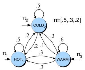
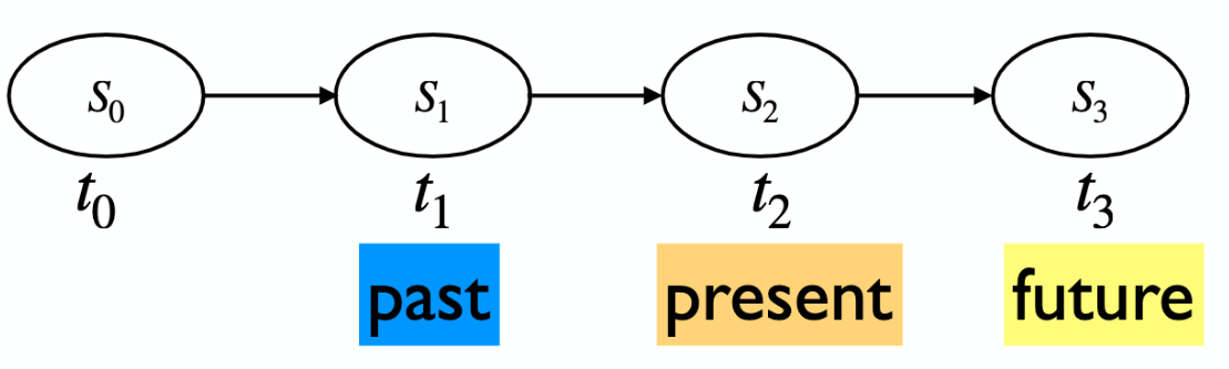
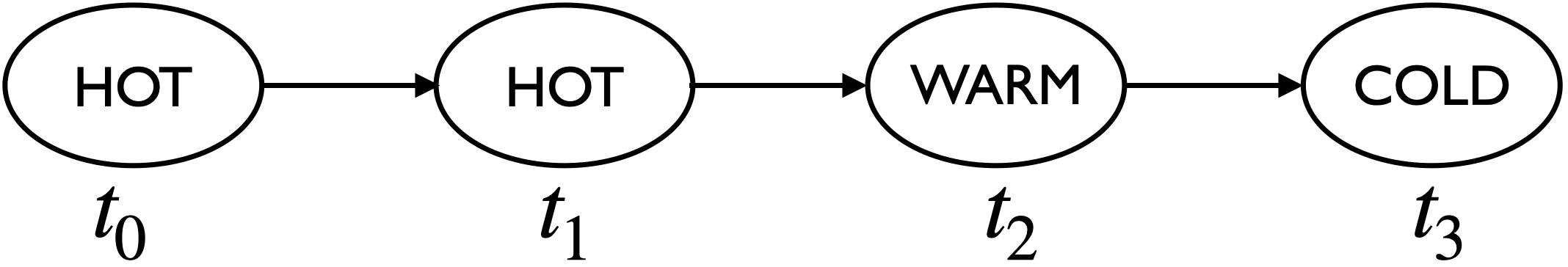
This is an unrolled version or a single realization of a Markov chain.
3.1 Discrete Markov chain ingredients#
State space
We have discrete timesteps: \(t = 0, t = 1, \dots\).
State space: We have a finite set of possible states we can be in at time \(t\)
Represent the unique observations in the world.
We can be in only one state at a given time.
In our toy example, the state space \(S = \{HOT, COLD, WARM\}\).
Initial probability distribution over states
State space: \(S = \{\text{HOT, COLD, WARM}\}\),
We could start in any state. The probability of starting with a particular state is given by an initial discrete probability distribution over states. In our toy example,
$\(\pi_0 = \begin{bmatrix} P(\text{HOT at time 0}) & P(\text{COLD at time 0}) & P(\text{WARM at time 0}) \end{bmatrix} = \begin{bmatrix} 0.5 & 0.3 & 0.2 \end{bmatrix}\)$
Transition probability matrix
State space: \(S = \{\text{HOT, COLD, WARM}\}\), initial probability distribution: \(\pi_0 = \begin{bmatrix} 0.5 & 0.3 & 0.2 \end{bmatrix}\)
Transition probability matrix \(T\), where each \(a_{ij}\) represents the probability of moving from state \(s_i\) to state \(s_j\), such that \(\sum_{j=1}^{n} a_{ij} = 1, \forall i\)
Note that each row sums to 1.0.
Each state has a probability of staying in the same state (or transitioning to itself).
Note that some people use the the notation where the columns sum to one.
You can think of transition matrix as a data structure used to organize all the conditional probabilities concisely and efficiently.
In our weather example state space, initial probability distribution, transition probability matrix are as follows:
Markov chain general definition
A set of \(n\) states: \(S = \{s_1, s_2, ..., s_n\}\)
A set of discrete initial probability distribution over states \(\pi_0 = \begin{bmatrix} \pi_0(s_1) & \pi_0(s_2) & \dots & \pi_0(s_n) \end{bmatrix}\)
Transition probability matrix \(T\), where each \(a_{ij}\) represents the probability of moving from state \(s_i\) to state \(s_j\), such that \(\sum_{j=1}^{n} a_{ij} = 1, \forall i\)
Homogeneous Markov chains
Transition probabilities tell you how your state probabilities are going to change over time.
In this course, we assume homogeneous Markov chain where transition probabilities are the same for all time steps \(t\).
3.2 Markov chains tasks#
What can we do with Markov chains?
Predict probabilities of sequences of states.
Compute probability of being in a particular state at time \(t\).
Stationary distribution: Find the steady state after running the chain for a long time.
Generation: generate sequences that follow the probabilities of the states.
You will be doing this in the lab.
3.2.1 Predict probabilities of sequences of states#
Given the Markov model: \(S = \{\text{HOT, COLD, WARM}\}\), \(\pi_0 = \begin{bmatrix} 0.5 & 0.3 & 0.2 \end{bmatrix}\), $\(T = \begin{bmatrix} 0.5 & 0.2 & 0.3\\ 0.2 & 0.5 & 0.3\\ 0.3 & 0.1 & 0.6\\ \end{bmatrix}\)$
Compute the probability of the sequences: HOT, HOT, WARM, COLD
Markov assumption: \(P(S_{t+1}\mid S_{0}, S_1, \dots, S_t) \approx P(S_{t+1} \mid S_t)\)
Your turn (Activity: 3 minutes)
Predict probabilities of the following sequences of states on your own.
COLD, COLD, WARM
HOT, COLD, HOT, COLD
Hint: If we want to predict the future, all that matters is the current state.
\(S = \{\text{HOT, COLD, WARM}\}\), \(\pi_0 = \begin{bmatrix} 0.5 & 0.3 & 0.2 \end{bmatrix}\), $\(T = \begin{bmatrix} 0.5 & 0.2 & 0.3\\ 0.2 & 0.5 & 0.3\\ 0.3 & 0.1 & 0.6\\ \end{bmatrix}\)$
3.2.2 Computing probability of being in a particular state at time \(t\)#
Example: Assuming that the time starts at 0, what is the probability of HOT at time 1?
What is the probability of HOT at time 1?
You can conveniently calculate it as the dot product between \(\pi_0\) and the first column of the transition matrix!
What is the probability of HOT, COLD, WARM at time 1?
You can get probabilities of all states HOT, COLD, WARM at time 1 by multiplying \(\pi_0\) by the transition matrix.
What is the probability of HOT, COLD, WARM at time 2?
Similarly can get probabilities of all states HOT, COLD, WARM at time 2 by multiplying \(\pi_1\) by the transition matrix. $\(\pi_2 = \pi_1T\)$
Probability of being in a particular state at time \(t\)
Calculate
Applying the matrix multiplication to the current state probabilities does an update to the state probabilities!
Let’s try it out with numpy.
pi_0 = np.array([0.5, 0.3, 0.2])  # initial state probability dist
T = np.array([[0.5, 0.2, 0.3], [0.2, 0.5, 0.3], [0.3, 0.1, 0.6]])  # transition matrix

print("Initial probability distribution over states: ", pi_0)
print("The transition probability matrix: \n", T)
Initial probability distribution over states:  [0.5 0.3 0.2]
The transition probability matrix:
 [[0.5 0.2 0.3]
 [0.2 0.5 0.3]
 [0.3 0.1 0.6]]
You can also get state probabilities at time \(t\) by multiplying pi_0 by the \(t^{th}\) power of the transition matrix. For example, you can estimate state probabilities at time step 18 as:
pi_0 @ np.linalg.matrix_power(T, 18)
array([0.34693878, 0.2244898 , 0.42857143])
import panel as pn
from panel import widgets
from panel.interact import interact
import matplotlib
from IPython.display import clear_output

pn.extension()

def f(time_steps):
    return f"State probabilities at time step {time_steps} (pi_{time_steps} = pi_0@T^{time_steps}) = {pi_0 @ np.linalg.matrix_power(T, time_steps)}"

interact(f, time_steps=widgets.IntSlider(name='Time step', start=0, end=30, step=2, value=0)).embed(max_opts=20)
Any interesting observations?
Break (~5 mins)#

❓❓ Questions for you#
Exercise 1.1 Select all of the following statements which are True (iClicker)#
(A) According to the Markov assumption the probability of being at a future state \(s_{t+1}\) is independent of the past states \(s_1\) to \(s_{t-1}\).
(B) In a Markov model, the sum of the conditional probabilities of transitioning from one state to all other states is equal to 1.0.
(C) In a Markov chain, the probabilities associated with self loops (staying in the same state) of all states should sum to one.
(D) Given \(\pi_0\) as initial state probability distribution, and \(T\) as transition matrix, we can calculate the probability distribution over states at time step \(k\) by multiplying \(\pi_0\) and \(T^k\).
Exercise 1.1: V’s Solutions!
(A) False. The probability of being in a future state is conditionally independent of the past given present.
(B) True
(C) False
(D) True
4. Markov chains tasks: Stationary distribution#
In the example above, after time step 18 or so, the state probabilities stopped changing!!
A stationary distribution of a Markov chain is a probability distribution over states that remains unchanged in the Markov chain as time progresses.
A probability distribution \(\pi\) on states \(S\) is stationary where the following holds for the transition matrix \(T\).
Why is this useful? This tells us about the behaviour of a Markov chain in the long run.
4.1 Stationary distribution: Toy Google Matrix example#
Imagine a toy internet with three webpages: Prajeet webpage, Varada webpage, MDS webpage
We’ll build a toy Markov model where the states are the above three web pages.
Transitions represent a web surfer clicking on a link and moving to a different page.
Questions we might want to answer?
What’s the behaviour of web surfers in the long run? Which webpages should get a high rank based on this behaviour?
import numpy as np

pi_0 = np.array([0.1, 0.5, 0.4])

T = np.array([[1/8, 3/8, 4/8],
              [1/8, 1/8, 6/8],
              [3/8, 1/8, 4/8]])
# Do all the rows sum to 1?

np.allclose(np.sum(T, axis=1), 1.0)
True
pi_0 @ np.linalg.matrix_power(T, 2)
array([0.28125, 0.18125, 0.5375 ])
pi_0 @ np.linalg.matrix_power(T, 30)
array([0.26190476, 0.19047619, 0.54761905])
pi_0 @ np.linalg.matrix_power(T, 31)
array([0.26190476, 0.19047619, 0.54761905])
def f(time_step):
    pi_time_step = pi_0 @ np.linalg.matrix_power(T, time_step)
    if not np.allclose(pi_time_step @ T, pi_time_step, atol=1e-04):
        s = f"NO STEADDY STATE YET\n {pi_time_step} @T != {pi_time_step}"
    else:
        s = f"STEADY STATE\n {pi_time_step}@T == {pi_time_step}"
    return s

interact(f, time_step=widgets.IntSlider(name='Time step', start=0, end=40, step=2, value=0)).embed(max_opts=20)
Seems like after the \(10^{th}\) time step, the state probabilities stay the same (within a tolerance).
So we have reached a steady state at \(\pi = \begin{bmatrix} 0.26190462 & 0.19047604 & 0.54761934 \end{bmatrix}\) such that
So the distribution \(\pi = \begin{bmatrix} 0.26190462 & 0.19047604 & 0.54761934 \end{bmatrix}\) is a stationary distribution in this case because we have \(\pi T = \pi\).
In the long run, MDS webpage is going to be visited more often followed by Prajeet’s webpage. Varada webpage is not going to be visited much 😀.
This is a high-level idea of Google’s famous PageRank algorithm. The question is how do we create the transition matrix? We’ll talk about this a bit in the next lecture.
4.2 Conditions for stationary distribution#
Stationary distribution looks like a desirable property.
Does a stationary distribution \(\pi\) exist and is it unique?
Under mild assumptions, a Markov chain has a stationary distribution.
Sufficient condition for existence/uniqueness is positive transitions.
\(P(s_t \mid s_{t-1}) > 0\)
But very often at least some of the transition probabilities are non-positive (e.g., zero).
Weaker sufficient conditions for existence/uniqueness
Irreducibility ✅
A finite Markov chain is irreducible if it is possible to get to any state from any state, potentially over multiple steps. This means that the state space is fully connected.
In other words, a finite Markov chain is irreducible if and only if its corresponding graph is strongly connected.
Aperiodicity ✅
A Markov chain is aperiodic if there’s no fixed cycle over which the transitions occur. Loosely speaking, this means the chain doesn’t fall into a repetitive loop over a specific number of steps.
4.3 Irreducibility and aperiodicity#
Consider the Markov chains shown below. Which chains are irreducible? Which ones are aperiodic?
A chain is irreducible if every state can be reached from every other state (possibly over multiple steps).
A chain is aperiodic if the system doesn’t fall into a fixed rhythm. Formally, the greatest common divisor (GCD) of return times to any state is 1.
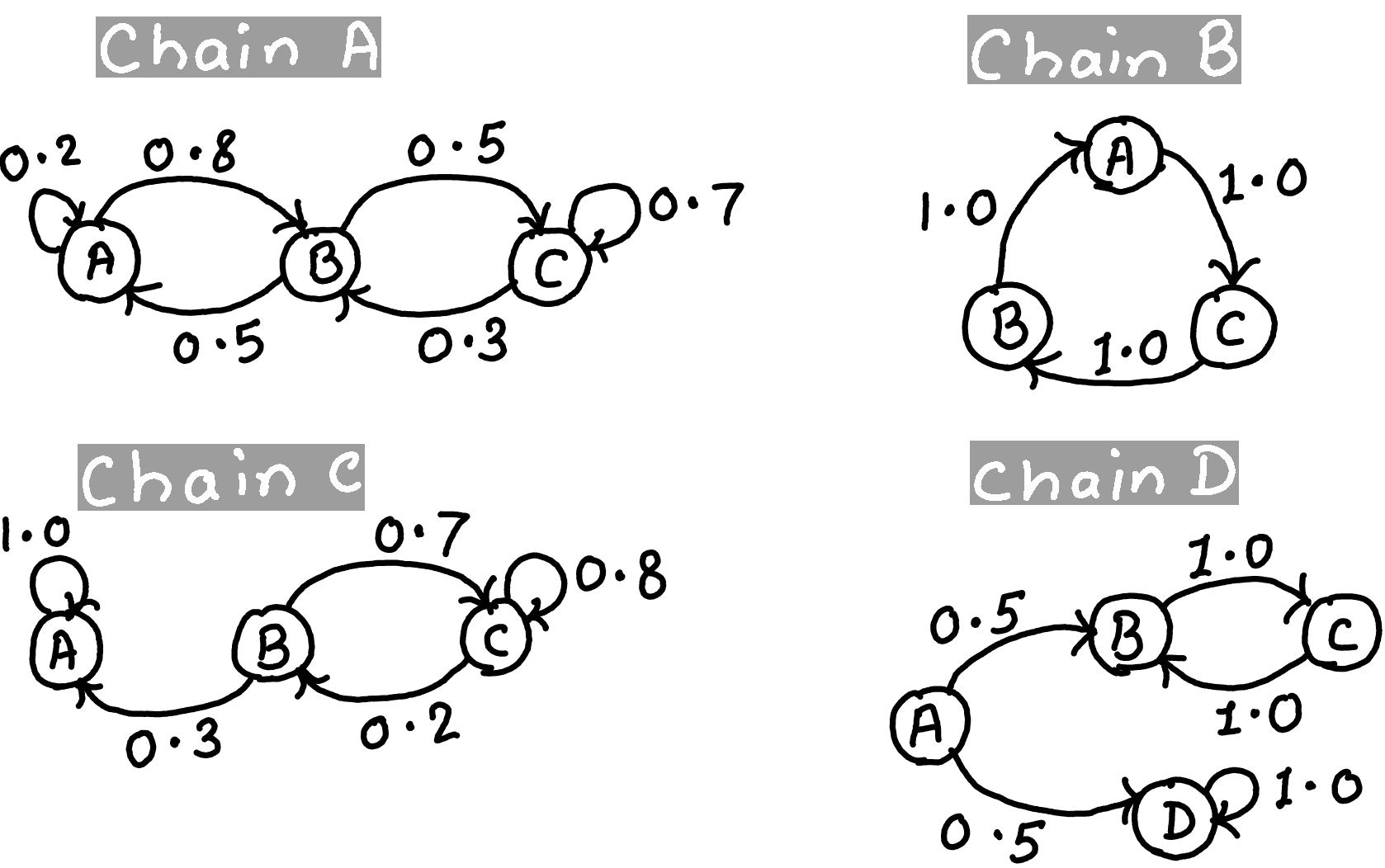
Chain |
Irreducible |
Aperiodic |
|---|---|---|
A |
✅ |
✅ |
B |
✅ |
❌ |
C |
❌ |
✅ |
D |
❌ |
❌ |
➡️ Irreducible and aperiodic Markov chains guarantee
The existence of a unique stationary distribution
That long-run behaviour doesn’t depend on initial state
In general:
Chain type |
Irreducible |
Aperiodic |
|---|---|---|
Self-loops everywhere, fully conntected chain |
✅ |
✅ |
Cycles (A \(\rightarrow\) B \(\rightarrow\) C \(\rightarrow\) A) |
✅ |
❌ |
Absorbing state only |
❌ |
✅ |
One-way transitions |
❌ |
❌ |
(Optional) Periodicity formal definition
A state in a Markov chain is periodic if the chain can return to the state only at multiples of some integer larger than 1. Thus, starting in state \(i\), the chain can return to \(i\) only at multiples of the period \(k\), and \(k\) is the largest such integer. State \(i\) is aperiodic if \(k = 1\) and periodic if \(k > 1\).
The period of a state is the greatest common divisor (GCD) of the number of steps in which you can return to it.
If the GCD > 1, the state is periodic
If the GCD = 1, the state is aperiodic
✅ Self-loops (e.g., A \(\rightarrow\) A) help break periodicity
❌ Fixed cycles (e.g., A \(\rightarrow\) B \(\rightarrow\) C \(\rightarrow\) A \(\rightarrow\) B \(\rightarrow\) C \(\rightarrow\) A) introduce periodicity
(Optional) Some ways to examine irreducibility
Power method: Compute higher powers of the transition matrix \(T^k\). If the chain is irreducible, for some \(k\), all the elements of \(T^k\) should be positive. This means there’s a positive probability of going from any state to any other state in k steps.
Check whether the graph is strongly connected or not.
Check out Kosaraju’s algorithm.
(Optional) Some ways to examine aperiodicity
Check diagonal of powers:
Take higher powers of the transition matrix \(T^k\).
If you find a power where all diagonal elements (which correspond to returning to the same state) are positive, it indicates that there’s no fixed cycle length for returning to any state, suggesting that the chain is aperiodic.
4.4 How to estimate the stationary distribution?#
Power iteration method
Multiply \(\pi_0\) by powers of the transition matrix \(T\) until the product looks stable.
Taking the eigenvalue decomposition of the transpose of the transition matrix \(\pi T=\pi\)
Through Monte Carlo simulation.
In some cases (not always) simply counting the occurrences (lab 1).
There are other ways too!
(Optional) Eigendecomposition to get stationary distribution
Note that \(\pi T = \pi\) looks very similar to the eigenvalue equation \(Av = \lambda v\) for eigenvalues and eigenvectors, with \(\lambda = 1\).
If you transpose the matrix
In other words, if we transpose the transition matrix and take its eigendecomposition, the eigenvector with eigenvalue 1 is going to be the stationary distribution.
If there are multiple eigenvectors with eigenvalue 1.0, then the stationary distribution is not unique.
❓❓ Questions for you#
Exercise 1.2: Select all of the following statements which are True#
(A) For a stationary distribution, the initial state probability distribution \(\pi_0\) must satisfy \(\pi_0T \approx \pi_0\).
(B) If a state has only one possible transition, the transition probability for that transition would be 1.0.
(C) If each row in the transition matrix of a Markov chain has only one possible transition, the chain would be deterministic.
(D) If we have a self loop transition with probability 1.0 for state A in a Markov chain and we happen to be at state A, the chain is going to get stuck in that state forever.
Exercise 1.2: V’s Solutions!
B, C, D
Final thoughts, summary, reflection#
We define a discrete Markov chain as
a set of finite states
an initial probability distribution over states
a transition probability matrix
We can do a number of things with Markov chains
Calculate the probability of a sequence.
Compute the probability of being in a particular state at time \(t\).
Calculate stationary distribution which is a probability distribution that remains unchanged in the Markov chain as time progresses.
Generate a sequence of states.
Learning Markov chains is just counting (next lecture).
Example applications of Markov chains in NLP (next lecture)
Language modeling
PageRank