Lecture 6: Introduction to self-attention and transformers

Lecture 6: Introduction to self-attention and transformers#

UBC Master of Data Science program, 2024-25

Attention is all you need!

Imports and LO#

Imports#

import IPython
from IPython.display import HTML, display

import matplotlib.pyplot as plt
import numpy as np
import pandas as pd
import torch
import torch.nn as nn
import torch.optim as optim

pd.set_option("display.max_colwidth", 0)

---------------------------------------------------------------------------
ImportError                               Traceback (most recent call last)
Cell In[1], line 7
      5 import numpy as np
      6 import pandas as pd
----> 7 import torch
      8 import torch.nn as nn
      9 import torch.optim as optim

File ~/miniforge3/envs/jbook/lib/python3.12/site-packages/torch/__init__.py:367
    365     if USE_GLOBAL_DEPS:
    366         _load_global_deps()
--> 367     from torch._C import *  # noqa: F403
    370 class SymInt:
    371     """
    372     Like an int (including magic methods), but redirects all operations on the
    373     wrapped node. This is used in particular to symbolically record operations
    374     in the symbolic shape workflow.
    375     """

ImportError: dlopen(/Users/kvarada/miniforge3/envs/jbook/lib/python3.12/site-packages/torch/_C.cpython-312-darwin.so, 0x0002): Library not loaded: @rpath/libgfortran.5.dylib
  Referenced from: <0B9C315B-A1DD-3527-88DB-4B90531D343F> /Users/kvarada/miniforge3/envs/jbook/lib/libopenblas.0.dylib
  Reason: tried: '/Users/kvarada/miniforge3/envs/jbook/lib/libgfortran.5.dylib' (duplicate LC_RPATH '@loader_path'), '/Users/kvarada/miniforge3/envs/jbook/lib/libgfortran.5.dylib' (duplicate LC_RPATH '@loader_path'), '/Users/kvarada/miniforge3/envs/jbook/lib/libgfortran.5.dylib' (duplicate LC_RPATH '@loader_path'), '/Users/kvarada/miniforge3/envs/jbook/lib/libgfortran.5.dylib' (duplicate LC_RPATH '@loader_path'), '/Users/kvarada/miniforge3/envs/jbook/lib/libgfortran.5.dylib' (duplicate LC_RPATH '@loader_path'), '/Users/kvarada/miniforge3/envs/jbook/lib/libgfortran.5.dylib' (duplicate LC_RPATH '@loader_path'), '/Users/kvarada/miniforge3/envs/jbook/lib/libgfortran.5.dylib' (duplicate LC_RPATH '@loader_path'), '/Users/kvarada/miniforge3/envs/jbook/lib/libgfortran.5.dylib' (duplicate LC_RPATH '@loader_path'), '/Users/kvarada/miniforge3/envs/jbook/lib/python3.12/site-packages/torch/lib/libgfortran.5.dylib' (no such file), '/Users/kvarada/miniforge3/envs/jbook/lib/python3.12/site-packages/torch/../../../libgfortran.5.dylib' (duplicate LC_RPATH '@loader_path'), '/Users/kvarada/miniforge3/envs/jbook/lib/python3.12/site-packages/torch/lib/libgfortran.5.dylib' (no such file), '/Users/kvarada/miniforge3/envs/jbook/lib/python3.12/site-packages/torch/../../../libgfortran.5.dylib' (duplicate LC_RPATH '@loader_path'), '/Users/kvarada/miniforge3/envs/jbook/bin/../lib/libgfortran.5.dylib' (duplicate LC_RPATH '@loader_path'), '/Users/kvarada/miniforge3/envs/jbook/bin/../lib/libgfortran.5.dylib' (duplicate LC_RPATH '@loader_path'), '/usr/local/lib/libgfortran.5.dylib' (no such file), '/usr/lib/libgfortran.5.dylib' (no such file, not in dyld cache)

Learning outcomes#

From this lecture you will be able to

Broadly explain the problem of vanishing gradients.
Broadly explain the limitations of RNNs.
Explain the idea of self-attention.
Describe the three core operations in self-attention.
Explain the query, key, and value roles in self-attention.
Explain the role of linear projections for query, key, and value in self-attention.
Explain transformer blocks.
Explain the advantages of using transformers over LSTMs.
Broadly explain the idea of multihead attention.
Broadly explain the idea of positional embeddings.

Attributions#

This material is heavily based on Jurafsky and Martin, Chapter 10.

❓❓ Questions for you#

Suppose you are training a vanilla RNN with one hidden layer.
- input representation is of size 200
- output layer is of size 200
- the hidden size is 100

Exercise 6.1: Select all of the following statements which are True (iClicker)#

(A) The shape of matrix $U$ between hidden layers in consecutive time steps is going to be $200 \times 200$.
(B) The output of the hidden layer (i.e., $h_t = tanh(W_{xh}x_{t} + W_{hh}h_{t-1} + b_{hh}$)) is going to be a $100$ dimensional vector.
(C) In bidirectional RNNs, if we want to combine the outputs of two RNNs with element-wise addition, the hidden sizes of the two RNNs have to be the same.
(D) Word2vec skipgram model is likely to suffer from the problem of vanishing gradients.
(E) In the forward pass, in each time step in RNNs, you calculate the output of the hidden layer by multiplying the input $x$ by the weight matrix $W$ or $W_{xh}$ and applying non-linearity.

Exercise 7.1: V’s Solutions!

B, C

1. Motivation#

What kind of neural network models are at the core of all state-of-the-art Generative AI models (e.g., BERT, GPT3, GPT4, Gemini, DALL-E, Llama, Github Copilot)?

Source

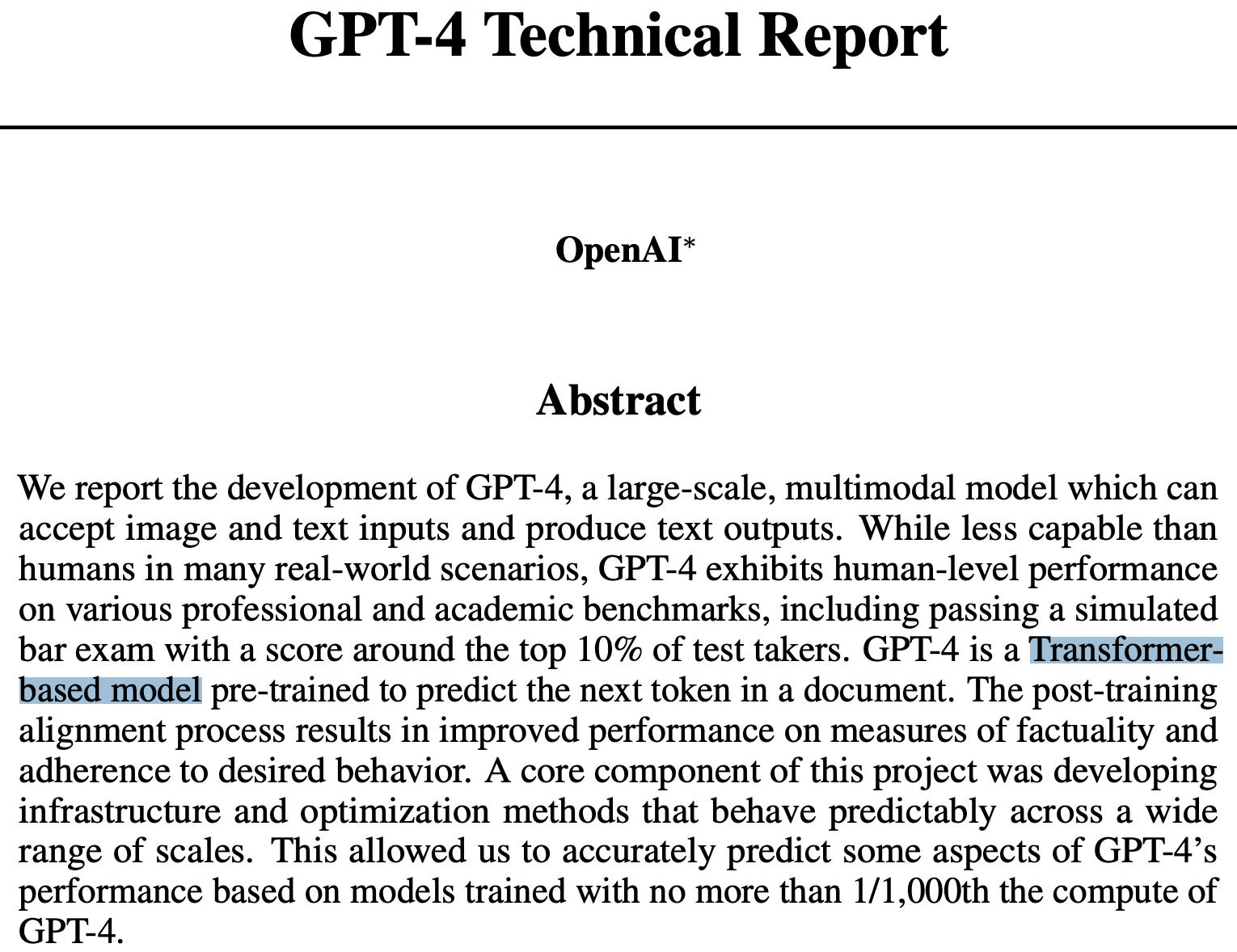
Source: GPT-4 Technical Report

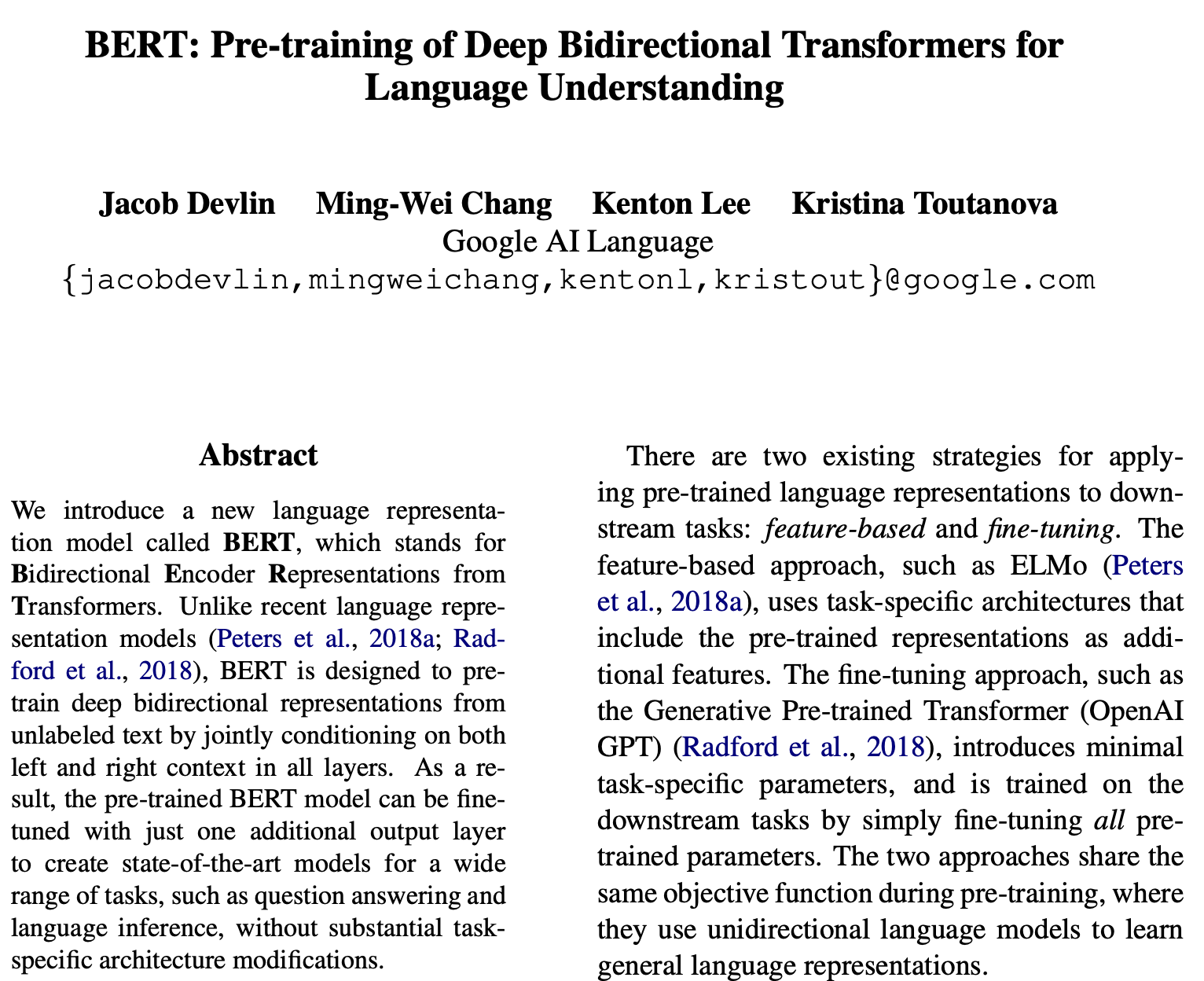
Source: BERT paper

Recall the properties we want when we model sequences.

[ ] Order matters
[ ] Variable sequence lengths
[ ] Capture long distance dependencies

What are some reasonable predictions for the missing words in the following sentences?

The students in the exam where the fire alarm is ringing __ really stressed.

The flies munching on the banana that is lying under the tree which is in full bloom __ really happy.

Markov models are able to represent time and handle variable sequence lengths. But they are unable to represent long-distance dependencies in text.

Are RNNs able to capture long-distance dependencies in text?

1.2 Problems with RNNs#

Conceptually, RNNs are supposed to capture long-distance dependencies in text. But in practice, you’ll hardly see people using vanilla RNNs because they are quite hard to train for tasks that require access to distant information. There are three main problems:

Hard to remember relevant information
Hard to optimize
Hard to parallelize

Problem 1: Hard to remember relevant information

In RNNs, the hidden layer and the weights that determine the values in the hidden layer are asked to perform two tasks simultaneously:
- Providing information useful for current decision
- Updating and carrying forward information required for future decisions
Despite having access to the entire previous sequence, the information encoded in hidden states of RNNs is fairly local.

In the following example:

The students in the exam where the fire alarm is ringing are really stressed.

Assigning high probability to is following alarm is straightforward since it provides a local context for singular agreement.
However, assigning a high probability to are following ringing is quite difficult because not only the plural students is distant, but also the intervening context involves singular constituents.
Ideally, we want the network to retain the distant information about the plural students until it’s needed while still processing the intermediate parts of the sequence correctly.

Problem 2: Hard to optimize

Another difficulty with training RNNs arises from the need to backpropagate the error signal back through time.
Recall that we learn RNNs with
- Forward pass
- Backward pass (backprop through time)
Computing new states and output in RNNs

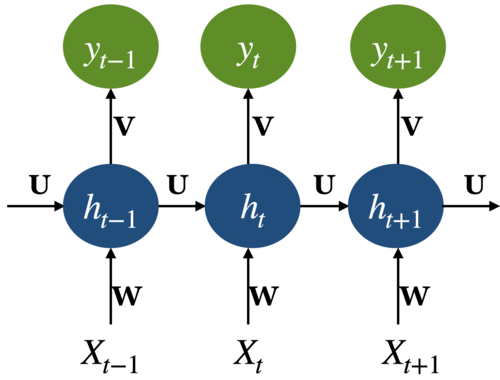
\[\begin{split} h_t = g(Uh_{t-1} + Wx_t + b_1)\\ y_t = \text{softmax}(Vh_t + b_2) \end{split}\]

Recall: Backpropagation through time

When we backprop with feedforward neural networks
- Take the gradient (derivative) of the loss with respect to the parameters.
- Change parameters to minimize the loss.
In RNNs we use a generalized version of backprop called Backpropogation Through Time (BPTT)
- Calculating gradient at each output depends upon the current time step as well as the previous time steps.

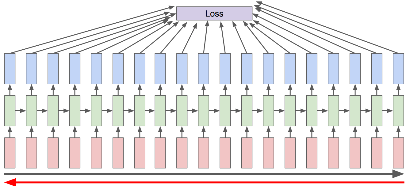
So in the backward pass of RNNs, we have to multiply many derivatives together, which very often results in
- vanishing gradients (gradients becoming very small and eventually driven to zero) in case of long sequences
If we have a vanishing gradient, we might not be able to update our weights reliably.
So we are not able to capture long-term dependencies, which kind of defeats the whole purpose of using RNNs.

To address these issues more complex network architectures have been designed with the goal of maintaining relevant context over time by enabling the network to learn to forget the information that is no longer needed and to remember information required for decisions still to come.
Most commonly used models are
- The Long short-term memory network (LSTM) (See this appendix on LSTMs.)
- Gated Recurrent Units (GRU)
That said, even with these models, for long sequences, there is still a loss of relevant information and difficulties in training.
Also, inherently sequential nature of RNNs/LSTMs make them hard to parallelize. So they are slow to train.

Problem 3: Hard to parallelize

Due to their inherently sequential nature

1.3 The Big Picture: Transformers#

Transformers are a powerful architecture for sequence modeling that eliminates the recurrence used in RNNs and LSTMs. Instead of processing tokens one-by-one, Transformers process all tokens simultaneously, making them highly efficient.
The key idea is to iteratively build contextualized vector representations of input tokens through multiple transformer layers. These representations capture not only the token’s own identity but also its relationships with other tokens in the sequence.
Compared to RNNs:
- Better at modeling long-range dependencies
- Easier to parallelize, speeding up training and inference
Transformers are the foundation of modern generative AI, powering models like:
- BERT, GPT-*
- DALL-E , SORA
- LLaMA (Meta), Bard (Google), Copilot (GitHub)

A look inside a transformer model

Let’s peek inside a common architecture used in large language models (LLMs):

The model consists of multiple stacked transformer blocks
e.g., GPT-3 has 96 layers!
Input: A sequence of tokens is converted into embeddings (word + positional (coming up soon))
Each transformer block contains:
- Multihead self-attention
- Feedforward layers
- Layer normalization
These blocks iteratively refine the representations to produce:
- Context-aware token representations
  e.g., the word “bank” will have different representations depending on its context
Output:
1. From transformer blocks: Rich contextual representations of each token
2. From final model head: A probability distribution over the vocabulary for the next token Below is a diagram showing this architecture in action:

Transformer Model

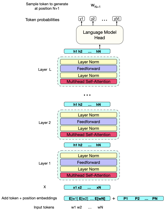
Source: Jurafsky & Martin’s Speech and Language Processing

Zooming In: The Transformer Block

Now that we’ve seen the big picture, let’s zoom in and examine a single Transformer block.

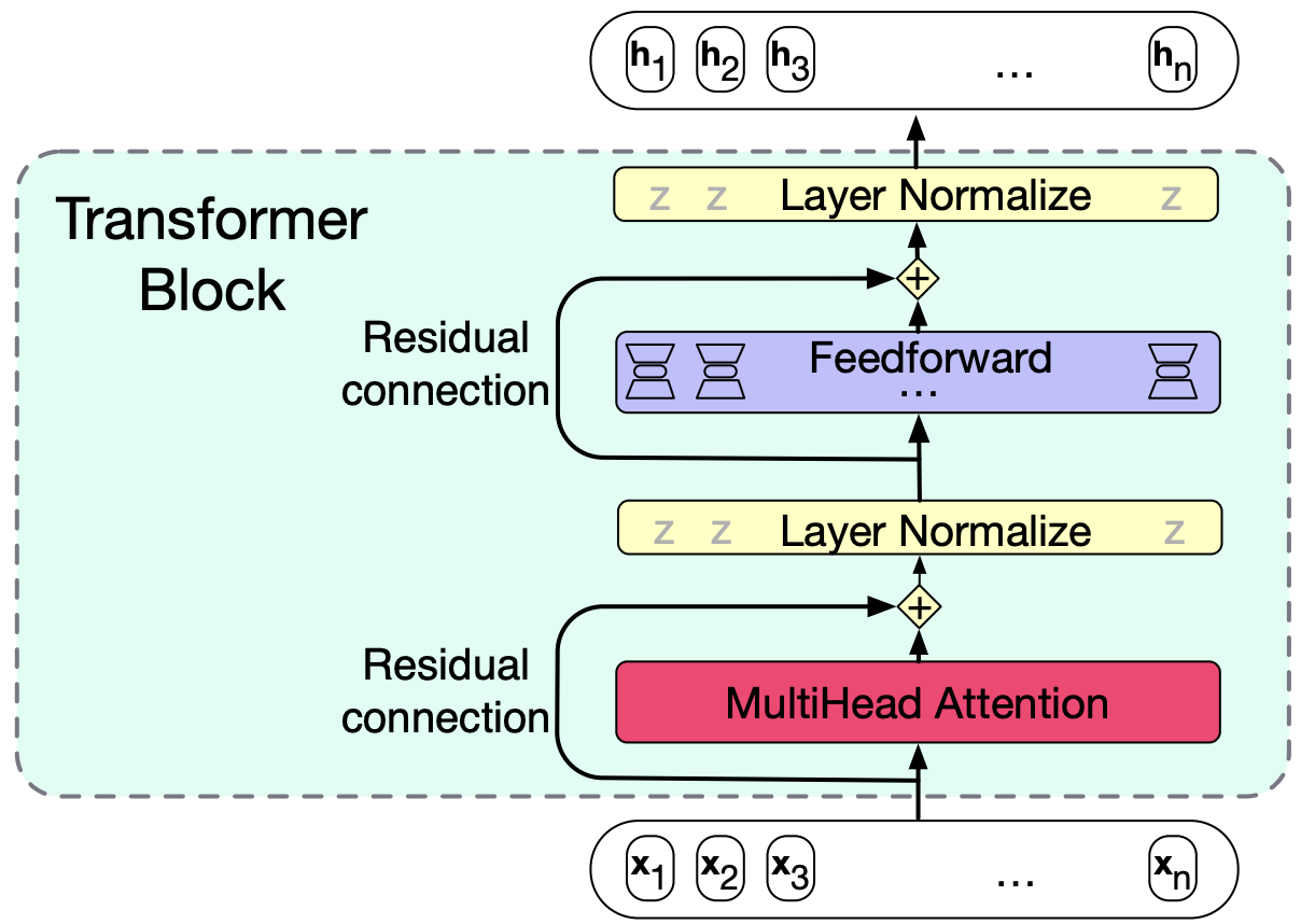
A Transformer block consists of the following components:

Multi-head self-attention layer: Learns relationships between tokens in a sequence.
Feedforward layer: Applies transformations independently to each token.
Residual connections: Help preserve information and improve gradient flow.
Layer normalization: Stabilizes and speeds up training.

Zooming in further: Multi-head self-attention

The multi-head attention layer is central to the transformer’s architecture.

It contains multiple self-attention heads running in parallel.
Each head can learn to focus on different aspects or relationships in the input sequence.

Two key innovations in transformers

There are two main innovations that make transformers effective:

Self-attention
Allows the model to weigh the importance of other tokens in the sequence when encoding a given token.
Positional embeddings/encodings
Since transformers do not process tokens sequentially, positional encodings are added to retain information about token order.

Let’s zoom in on self-attention.

2. Self-attention#

2.1 Intuition#

Biological motivation for self-attention

Count how many times the players wearing the white pass the basketball?

### An example of a state-of-the-art language model
url = "https://www.youtube.com/embed/vJG698U2Mvo"
IPython.display.IFrame(url, width=500, height=500)

When we process information, we often selectively focus on specific parts of the input, giving more attention to relevant information and less attention to irrelevant information. This is the core idea of attention.

Consider the examples below:

Example 1: She left a brief note on the kitchen table, reminding him to pick up groceries.
Example 2: The diplomat’s speech struck a positive note in the peace negotiations.
Example 3: She plucked the guitar strings, ending with a melancholic note.

The word note in these examples serves quite distinct meanings, each tied to different contexts.

To capture varying word meanings across different contexts, we need a mechanism that considers the wider context to compute each word’s contextual representation.
Self-attention is just that mechanism!
It allows us to look broadly into the context and tells us how to integrate the representations of context words to build representation of a word.
A question for you: why not use traditional word embeddings we have seen so far (like word2vec or GloVe)?

Let’s visualize self-attention, we’ll focus on how the word note is interpreted within its sequence.

She plucked the guitar strings , ending with a melancholic note .

Which words in the context are most relevant to note? Assign a qualitative weight (high or low) to each context word below.

note attending to She: low weight
note attending to plucked:
note attending to ending:
note attending to guitar:
note attending to strings:
note attending to melancholic:

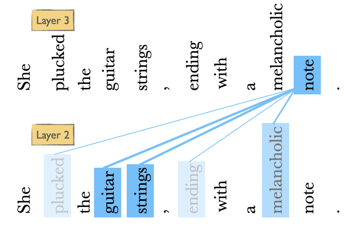
Self-attention mechanism allows a neural network model to ‘attend’ to different parts of the input data with varying degrees of focus.
We compare a token of our interest to a collection of other tokens in the context that reveal their relevance in the current context. (The relevance is denoted with the colour intensity in the diagram above.)
For each token in the sequence, we assign a weight based on how relevant it is to the token under consideration.
Calculate the output for the current token based on these weights.
It allows a network to directly extract and use information from arbitrarily large contexts without the need to pass it through intermediate recurrent connections as in RNNs.

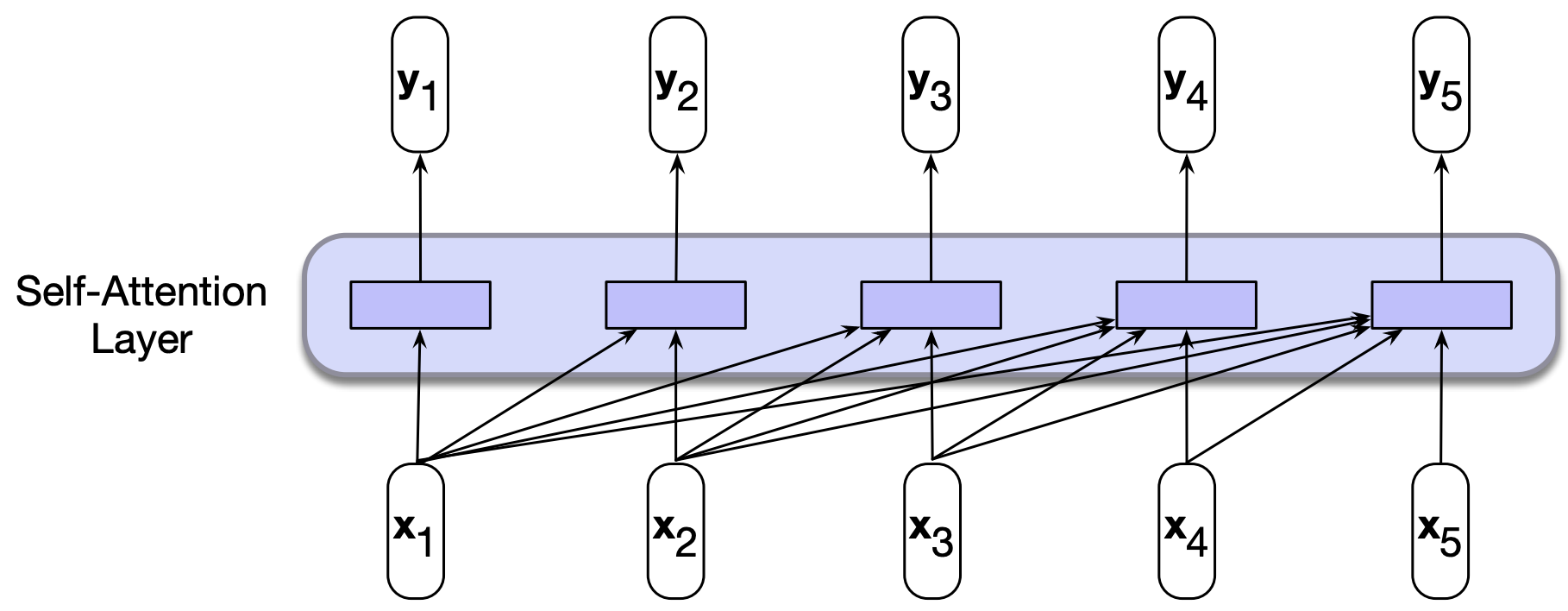
Below is a single backward looking self-attention layer which maps sequences of input vectors $(x_1, \dots, x_n)$ to sequences of output vectors $(y_1, \dots, y_n)$ of the same length.
When processing an item at time $t$, the model has access to all of the inputs up to and including the one under consideration.
It does not have access to the input beyond the current one.
Note that unlike RNNs or LSTMs, each computation can be done independently; it does not depend upon the previous computation which allows us to easily parallelize forward pass and the training of such models.

Source

2.2 The key operations in self-attention#

To determine the weights of various tokens in the context during self-attention’s output calculation for a specific token, we follow three key operations

Calculate scores with dot products between tokens
Apply softmax to derive a probability distribution
Compute a weighted sum based on the scores for all observed inputs

Now, let’s break down these operations step by step.

Example: Calculating the output $y$ for the token note in the given context

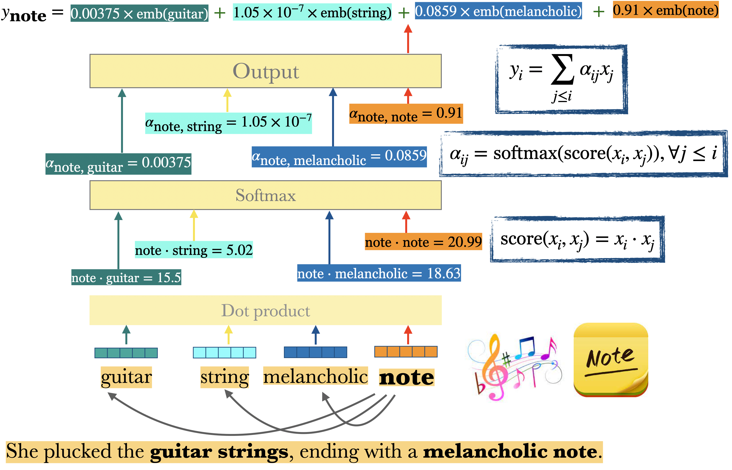
To generalize, in order to calculate the output $y_i$

We score token $x_i$ with all previous tokens $x_j$ by taking the dot product between them. $$\text{score}(x_i, x_j) = x_i \cdot x_j$$
We apply $\text{softmax}$ on these scores to get probability distribution over these scores. $$\alpha_{ij} = \text{softmax}(\text{score}(x_i \cdot x_j)), \forall j \leq i$$
The output is the weighted sum of the inputs seen so far, where the weights correspond to the $\alpha$ values calculated above. $$y_i = \sum_{j \leq i} \alpha_{ij}x_j$$
The final output vector incorporates the information from all relevant parts of the sentence, weighted by their relevance to the target word “note”.

These three operations outline the core of an attention-based approach. These operations can be carried out independently for each input allowing easy parallelism. Now, let’s introduce additional bells and whistles to make it trainable.

2.3 Query, Key, and Value Roles#

In the process of calculating outputs for each input token, each token plays three roles: Query, Key, and Value.

What do these roles represent?

Remember, our goal is to create contextual representations for tokens in the sequence. For each word, we want to figure out:

Which tokens in the context are important for me?
Which tokens should I attend to?

Let’s consider some possible Query, Key, and Value roles using the example sequence:

guitar string melancholic note

Token	Key	Value	Query
guitar	instrument, noun, object	a musical instrument	what am I connected to or describing?
string	part of an object, noun	a thin part of an instrument	what do I belong to?
melancholic	emotion, adjective, mood descriptor	sad, emotional, somber	what do I describe?
note	sound, noun, musical output	a sound or tone produced	where did I come from? what defines me?

melancholic will attend strongly to note, because its query is “what do I describe?” and note’s key is “sound, noun, musical output”.
string will likely attend to guitar, since its query is about belonging, and guitar’s key signals it as the larger object.
note may attend to both string and melancholic, blending physical and emotional context into its representation.

Once we have the attention weights for all tokens, we compute contextual representations by combining the value vectors, weighted by these attention scores.

In summary, each role reflects a different perspective of the same token:

Key: “What do I offer to others?” $\rightarrow$ e.g., emotion, adjective, mood descriptor
Value: “What is my actual content or meaning?” $\rightarrow$ e.g., sad, emotional, somber
Query: “What am I looking for in others?” $\rightarrow$ e.g., What do I describe?

Self-attention activity

TBD

For these three roles, the Transformer introduces three learnable weight matrices: $W^Q$, $W^K$, and $W^V$. These weights are used to project each input vector $x_i$ into its role as a query, key, or value.

\[ q_i = W^Q x_i \]

\[ k_i = W^K x_i \]

\[ v_i = W^V x_i \]

Each token’s input embedding $x_i$ is transformed three times, once for each role, using these matrices. This allows the model to learn how each token should behave in different roles, based on the task and data.

For now, let’s assume that all of these weight matrices project to the same dimensional space, so the resulting vectors $q_i$, $k_i$, and $v_i$ are all of equal size.

With these projections our equations become:

We score the $x_i$ with all previous tokens $x_j$ by taking the dot product between $x_i$’s query vector $q_i$ and $x_j$’s key vector $k_j$:
$$\text{score}(x_i, x_j) = q_i \cdot k_j$$
The softmax calculation remains the same but the output calculation for $y_i$ is now based on a weighted sum over the projected vectors $v$: $$y_i = \sum_{j \leq i} \alpha_{ij}v_j$$

Source

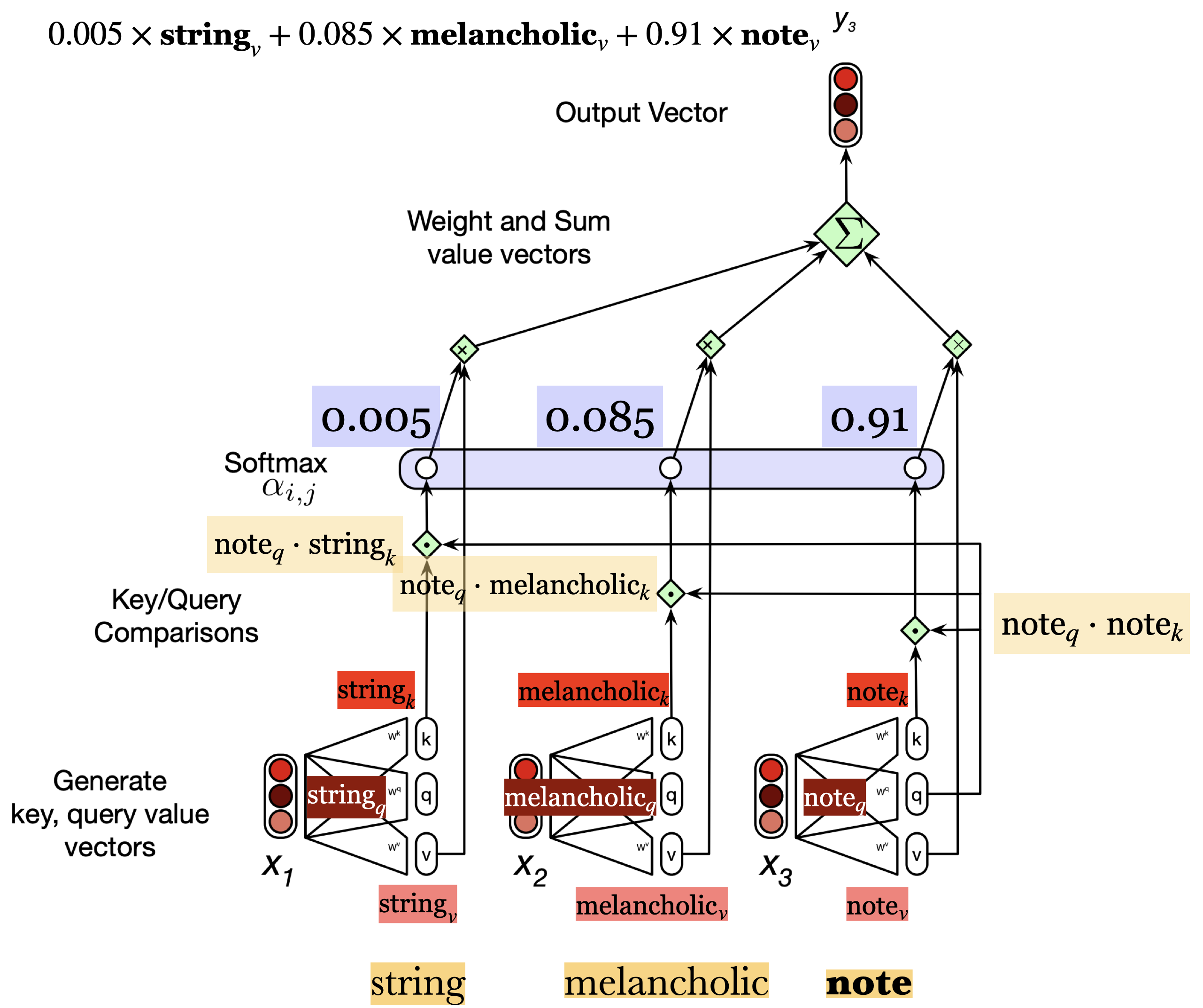
Let’s calculate the output of note in the following sequence with $K, Q, V$ matrices.

string melancholic note

Suppose input embedding is of size 300.
Suppose the projection matrices $W^k, W^q, W^v$ are of shape $300 \times 100$.
So word$_k$, word$_q$, word$_v$ provide 100-dimensional projections of each word corresponding to the key, query and value roles. For example, note$_k$, note$_q$, bite$_v$ represent 100-dimensional projections of the word note corresponding to its key, query, and value roles, respectively.
The dot products will be calculated between the appropriate query and key projections. In this example, we will calculate the following dot products:
- $\text{note}_q \cdot \text{string}_k$
- $\text{note}_q \cdot \text{melancholic}_k$
- $\text{note}_q \cdot \text{note}_k$
We apply softmax on these dot products. Suppose the softmax output in this toy example is

(14)#\[\begin{bmatrix} 0.005 & 0.085 & 0.91 \end{bmatrix}\]

So we have weights associated with three input words: string (0.005), melancholic (0.085) and note (0.91)
We can calculate the output as the weighted sum of the inputs. Here we will use the value projections of the inputs: $0.005 \times \text{string}_v + 0.085 \times \text{melancholic}_v + 0.91 \times \text{note}_v$
Since we will be adding 100 dimensional vectors (size of our projections), the dimensionality of the output $y_3$ is going to be 100.

Source

Scaling the dot products

The result of a dot product can be arbitrarily large and exponentiating such values can lead to numerical issues and problems during training.
So the dot products are usually scaled before applying the softmax.
The most common scaling is where we divide the dot product by the square root of the dimensionality of the query and the key vectors. $$\text{score}(x_i, x_j) = \frac{q_i \cdot k_j}{\sqrt{d_k}}$$

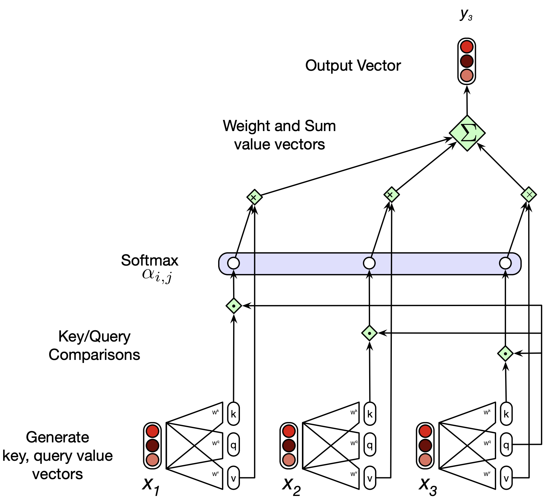
Here is a schematic of all computations involved in self-attention.

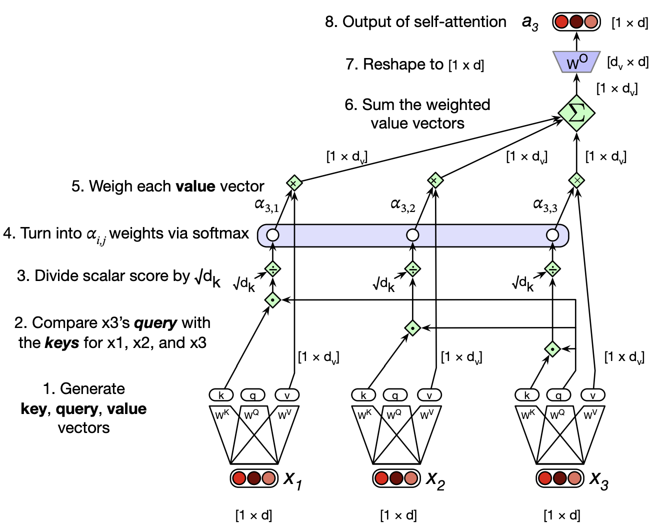
This is how we calculate a single output of a single time step $i$.

Would the output calculation at different time steps be dependent upon each other?

2.4 Efficient attention weight computation#

Let’s say we have an input sequence of $N$ tokens, where each token is represented by a $d$-dimensional embedding. We can stack all of these into a single matrix:

$X \in \mathbb{R}^{N \times d}$: Each row of $X$ is the embedding of one token in the sequence.

To calculate self-attention, we first project $X$ into three new matrices using learned weight matrices:

$W^Q \in \mathbb{R}^{d \times d_k}$: weight matrix for queries
$W^K \in \mathbb{R}^{d \times d_k}$: weight matrix for keys
$W^V \in \mathbb{R}^{d \times d_v}$: weight matrix for values

We compute:

\[ Q = X W^Q \quad \text{(Query matrix: } N \times d_k \text{)} \]

\[ K = X W^K \quad \text{(Key matrix: } N \times d_k \text{)} \]

\[ V = X W^V \quad \text{(Value matrix: } N \times d_v \text{)} \]

With these matrices, we can now calculate all pairwise query-key scores simultaneously using matrix multiplication:

\[ Q \times K^\top \]

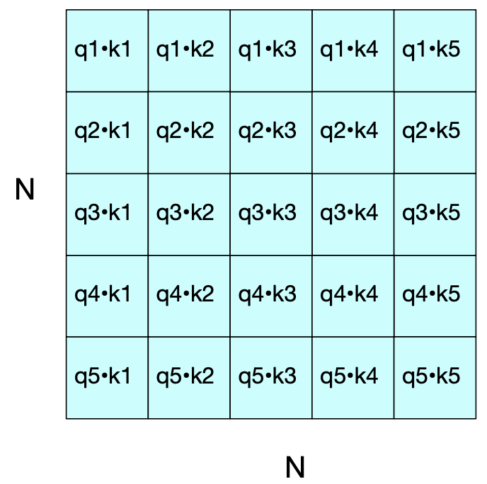
This gives us a matrix of dot products where each entry represents how much attention a token (as a query) should pay to another token (as a key).

\[ \text{Attention}(Q, K, V) = \text{softmax}\left(\frac{QK^\top}{\sqrt{d_k}}\right) V \]

$QK^\top$ computes dot products between all query-key pairs (shape: $N \times N$)
The softmax normalizes scores across each row (i.e., for each query token)
The result is a weighted sum of value vectors, producing the contextualized embeddings

Attention mask

What’s the issue with the $QK^\top$ calculation above?
- It computes scores for all token pairs, including future tokens.
- In language modeling, we want to predict the next word based only on previous words, not words that come later.
Why is this a problem?
- If each token can “peek” at future tokens during training, the model would be cheating, it sees the answer before predicting it.
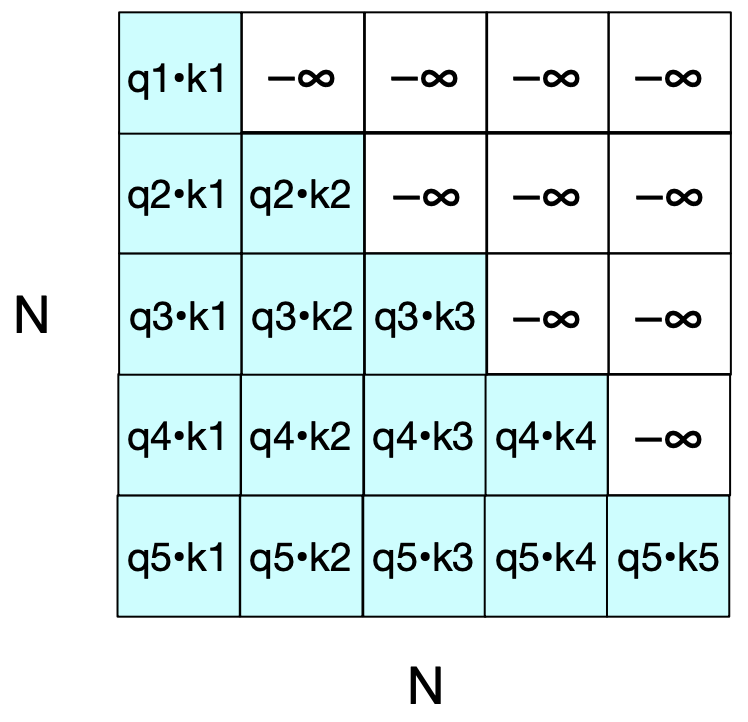
Solution: Use an attention mask!
- A mask is applied to the $QK^\top$ matrix to block out positions corresponding to future tokens.
- These positions are set to $-\infty$ (or a large negative number), so after applying softmax, their weights become zero.

Source

Break#

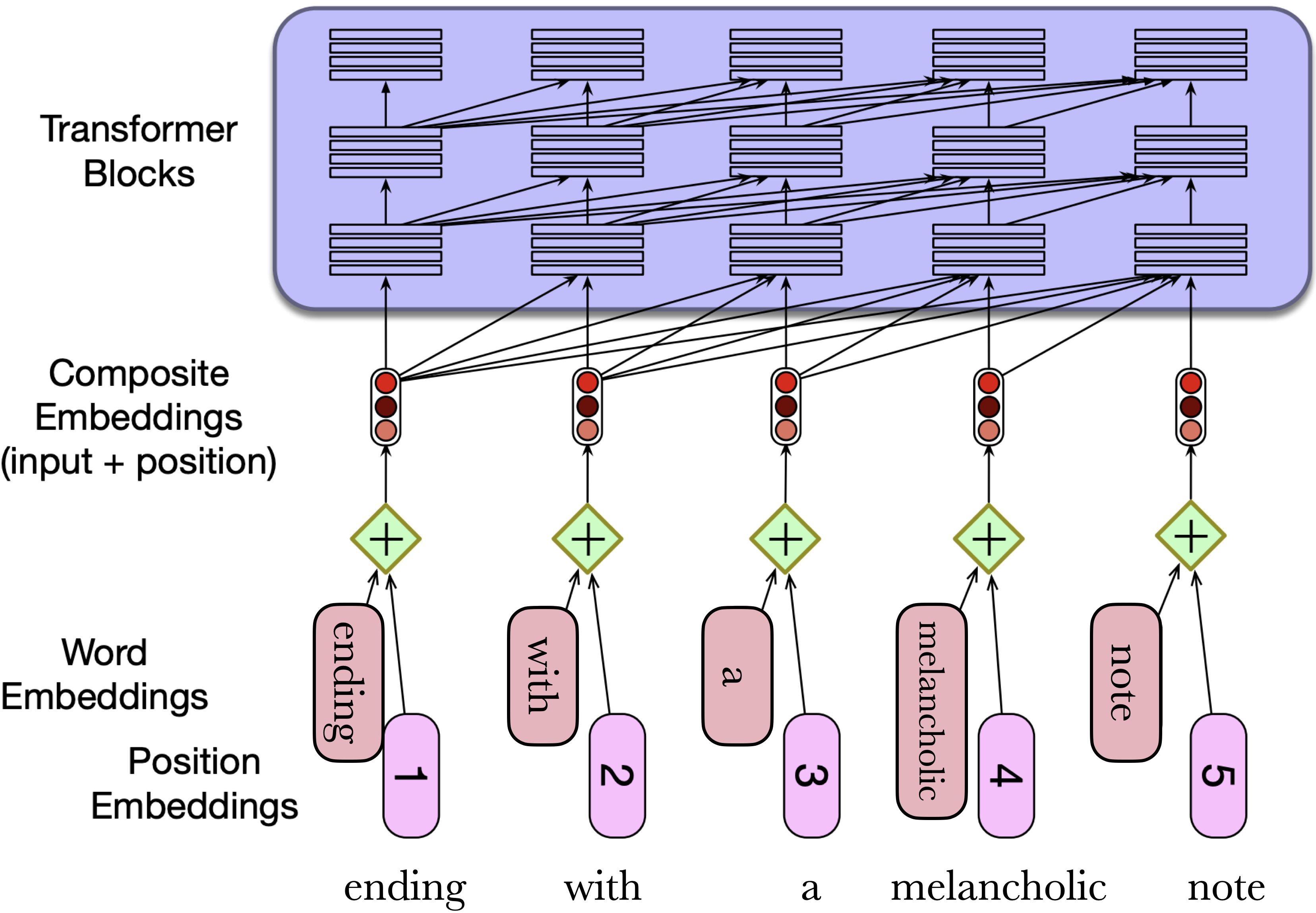
3. Positional embeddings#

Also called positional encodings.
Are we capturing word order when we calculate $y_3$? In other words, if you scramble the order of the inputs, will you get exactly the same answer for $y_3$?

Self-attention doesn’t naturally know the order of tokens. They treat input as a bag of words. Unlike RNNs or CNNs, which process inputs sequentially or locally, Self-attention process all tokens in parallel. That’s powerful, but also means they need extra help to understand the order of the sentence.

How can we capture word order and positional information?

A simple solution is positional embeddings! They help us figure our where in the sequence the token is.
- Without positional info: “guitar string” and “string guitar” look the same to the model.
- With it: The model learns: “guitar” came first, and that matters.
To produce an input embedding that captures positional information,
- We create positional embedding for each position (e.g., 1, 2, 3, …)
- We add it to the corresponding input embedding
- The resulting embedding has some information about the input along with its position in the text
Where do we get these positional embeddings? The simplest method is to start with randomly initialized embeddings corresponding to each possible input position and learn them along with other parameters during training.

4. Multi-head attention#

Different words in a sentence can relate to each other in many different ways simultaneously.
Consider the sentence below.

The cat was scared because it didn’t recognize me in my mask.

Let’s look at all the dependencies in this sentence.

import spacy
from spacy import displacy

nlp = spacy.load("en_core_web_md")

doc = nlp("The cat was scared because it did n't recognize me in my mask .")
displacy.render(doc, style="dep")

So a single attention layer usually is not enough to capture all different kinds of parallel relations between inputs.
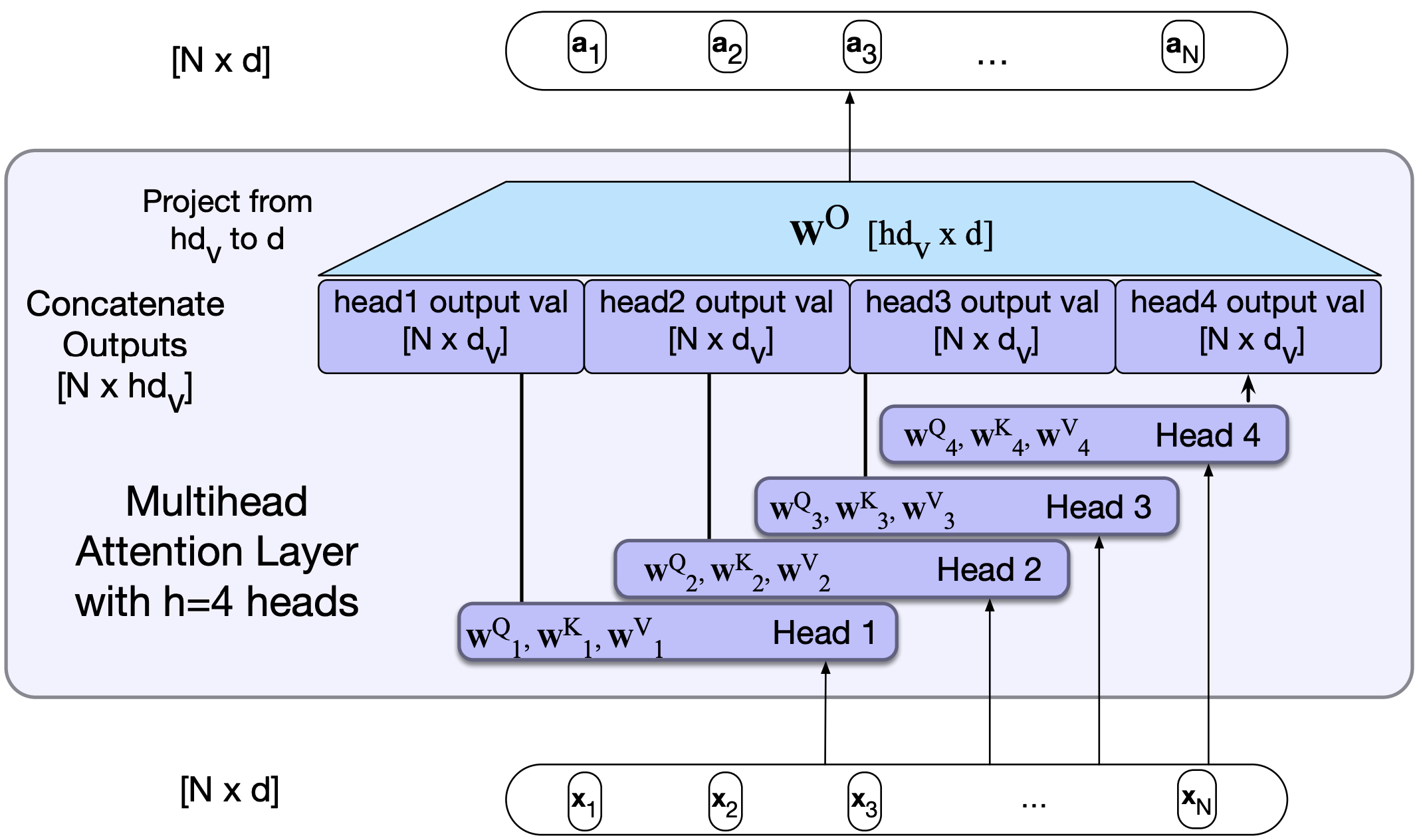
Transformers address this issue with multihead self-attention layers.
These self-attention layers are called heads.
They are at the same depth of the model, operate in parallel, each with a different set of parameters.
The idea is that with these different sets of parameters, each head can learn different aspects of the relationships that exist among inputs.

(15)#\[\begin{equation} \begin{split} MultiHeadAttn(X) &= (\text{head}_1 \oplus \text{head}_2 \dots \oplus \text{head}_h)W^O\\ Q &= XW_i^Q ; K = XW_i^K ; V = XW_i^V\\ \text{head}_i &= SelfAttention(Q,K,V) \end{split} \end{equation}\]

Source

Visualization of multi-head attention

Similar to RNNs you can stack self-attention layers or multihead self-attention layers on the top of each other.
Let’s look at this visualization which shows where the attention of different attention heads is going in multihead attention.
- Multi-head attention interactive visualization

5. Transformer blocks#

In many advanced architectures, you will see transformer blocks which consists of
- The multi-head self-attention layer
- Feedforward layer
- Residual connections
- Layer Norm

Source

Feedforward layer

The feedforward layer is a fully-connected 2-layer network (i.e., one hidden layer, two weight matrices)
The weights are the same for each token position $i$ , but are different from layer to layer.

Residual connections

Connections that pass information from a lower layer to a higher layer without going through the intermediate layer.
Residual connections help the transformer preserve useful information, train deeper networks, and let each layer build on top of the previous ones, rather than starting over.
They are implemented simply by adding a layer’s input vector to its output vector before passing it forward.
Typically, residual connections are used with both attention and feedforward layers.

Layer normalization or layer norm

The summed vectors are normalized in this layer.
Layer norm applies something similar to StandardScaler so that the mean is 0 and standard deviation is 1 in the vector.
This is done to keep the values of a hidden layer in a range that facilitates gradient-based training.
For each poisition, the input is a $d-$dimensional vector and the output is a normalized $d-$dimensional vector.

Putting it all together:

Here is the function computed by a transformer.

\[\begin{split}\begin{align} T^1 &= \text{SelfAttention}(X)\\ T^2 &= X + T^1\\ T^3 &= \text{LayerNorm}(T^2)\\ T^4 &= \text{FFN}(T^3)\\ T^5 &= T^4 + T^3\\ H &= \text{LayerNorm}(T^5) \end{align} \end{split}\]

The input and output dimensions of these layers are matched so that they can be stacked.
Each token $x_i$ at the input to the block has dimensionality $d$.
The input $X$ and output $H$ are both of shape $N \times d$, where $N$ is the sequence length.

5.1 Language models with transformers#

Language models with single transformer block

The job of the language modeling head is to take the output $h_N^{L}$, which represents the output token embedding at position $N$ from the final block $L$, and use it to predict the upcoming word at position $N+1$
The shape of $h_N^{L}$ is $1 \times d$.
We project it to the logit vector of shape $1 \times V$, where $V$ is the vocabulary size.
Recall the embedding layer at the beginning of the network. The input to our network is one-hot-encoding of tokens and the weight matrix between input and embedding layer is $V \times d$
Since this linear layer performs the reverse mapping from $d$ dimensions to $V$ dimensions, it is referred to as unembedding layer.

Source

Language models with multiple transformer blocks

Transformers for large language models stack many of these blocks.
T5 language model or GPT-3 small language models stack 12 such blocks.
GPT-3 large stacks 96 blocks.

Source

Final comments and summary#

Transformers are non-recurrent networks based on self-attention.
There are two main components of transformers:
- A self-attention layer maps input sequences to output sequences of the same length using attention heads which model how the surrounding words are relevant for the processing of the current word.
- Positional embeddings/encodings
A transformer block consists of a multi-head attention layer, followed by a feedforward layer with residual connections and layer normalizations. These blocks can be stacked together to create powerful networks.

Resources#

Attention-mechanisms and transformers are quite new. But there are many resources on transformers. I’m listing a few resources here.

Attention is all you need
Transformers
3Blue1Brown has recently released some videos on transformers
- But what is a GPT? Visual intro to transformers | Chapter 5, Deep Learning
- Attention in transformers
The Illustrated Transformer
Transformers documentation
A funny video: I taught an AI to make pasta
BERT

Coming up: Some applications of transformers

Lecture 6: Introduction to self-attention and transformers

Contents

Lecture 6: Introduction to self-attention and transformers#

Imports and LO#

Imports#

Learning outcomes#

Attributions#

❓❓ Questions for you#

Exercise 6.1: Select all of the following statements which are True (iClicker)#

1. Motivation#

1.2 Problems with RNNs#

1.3 The Big Picture: Transformers#

2. Self-attention#

2.1 Intuition#

2.2 The key operations in self-attention#

2.3 Query, Key, and Value Roles#

2.4 Efficient attention weight computation#

Break#

3. Positional embeddings#

4. Multi-head attention#

5. Transformer blocks#

5.1 Language models with transformers#

Final comments and summary#

Resources#