
Lecture 3: Introduction to Hidden Markov Models (HMMs)#
UBC Master of Data Science program, 2024-25
Imports, LO#
Imports#
import os
import re
import sys

import matplotlib.pyplot as plt
import numpy as np
import pandas as pd

import sys
sys.path.append(os.path.join(os.path.abspath(".."), "code"))
from plotting_functions import *
import IPython
from IPython.display import HTML, display
Learning outcomes#
From this lesson you will be able to
explain the motivation for using HMMs
define an HMM
state the Markov assumption in HMMs
explain three fundamental questions for an HMM
apply the forward algorithm given an HMM
explain supervised training in HMMs
1. Motivation#
1.1 Speech recognition#
Speech recognition is a key component of virtual assistants like Siri, Alexa, and Google Assistant. When we speak to them, they must:
Convert the audio signal into text.
Understand the intent.
Return a response.
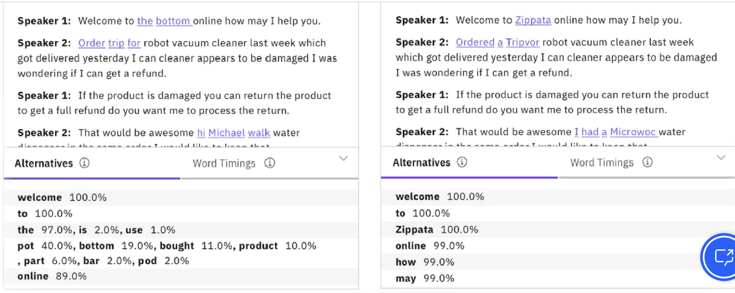
All steps have their own challenges but the first step of converting the audio signal into text (speech recognition) is especially difficult. Here’s an example where
Two speech recognizers transcribe the same utterance differently.
Small errors (e.g., “bottom” vs “Zippata”) drastically change meaning.
In speech recognition:
Input: an audio sequence (i.e., a time series of sound waves)
Output: a sequence of words or phonemes
Phonemes are the smallest units of sound. Examples:
tree \(\rightarrow\) T R IY
stats \(\rightarrow\) S T AE T S
eks \(\rightarrow\) E K S
There are approximately 40 to 45 phonemes in North American English, depending on the dialect.
Activity
Say the following phrases out loud:
stop
of value
tree
Which ones feel easier or smoother to say? Which one feels like it requires more effort?
Language is full of patterns. In English, some phoneme transitions occur more frequently and naturally than others:
/s/ \(\rightarrow\) /t/ (stop, best) is common
/t/ \(\rightarrow\) /r/ (tree, train) is also common
/f/ \(\rightarrow\) /v/ is less common and harder to pronounce
Our goal is to effectively model these kinds of transition.
Discussion question
Is it possible to use the ML models such as logistic regression or SVMs to solve this kind of problem?
Speech is sequential. Each word or phoneme often depends on the previous ones. The same applies to both word sequences and phoneme sequences.
Traditional machine learning models like decision trees or support vector machines (SVMs) do not naturally model these sequential dependencies. They treat each input independently.
For speech recognition, we need sequence models, models that explicitly account for transitions between units (words or phonemes).
In this lecture, we’ll explore Hidden Markov Models (HMMs), a class of models specifically designed for working with sequences like speech and language.
Speech recognition APIs
Python has many wrappers for speech APIs (e.g.,
SpeechRecognition) which can let you access these APIs.Some APIs:
Google, IBM, Microsoft, Wit.ai, OpenAI Whisper
Often need API keys, some work offline (e.g., CMU Sphinx)
(Optional) Demo
import sounddevice as sd
from scipy.io.wavfile import write
import whisper
import numpy as np
import IPython.display as ipd

# Record Audio
def record_audio(filename="output.wav", duration=5, fs=44100):
    print(f"Recording for {duration} seconds...")
    recording = sd.rec(int(duration * fs), samplerate=fs, channels=1, dtype='int32')
    sd.wait()
    write(filename, fs, recording)
    print(f"Saved recording as {filename}")
    return filename

# Transcribe Audio Using Whisper
def transcribe_audio(filename, model_size="base"):
    print("Loading Whisper model...")
    model = whisper.load_model(model_size)
    print("Transcribing...")
    result = model.transcribe(filename)
    print("Transcription:", result["text"])
    return result["text"]
---------------------------------------------------------------------------
ImportError                               Traceback (most recent call last)
Cell In[2], line 2
      1 import sounddevice as sd
----> 2 from scipy.io.wavfile import write
      3 import whisper
      4 import numpy as np

File ~/miniforge3/envs/jbook/lib/python3.12/site-packages/scipy/io/__init__.py:97
      1 """
      2 ==================================
      3 Input and output (:mod:`scipy.io`)
   (...)
     94    ParseArffError
     95 """
     96 # matfile read and write
---> 97 from .matlab import loadmat, savemat, whosmat
     99 # netCDF file support
    100 from ._netcdf import netcdf_file, netcdf_variable

File ~/miniforge3/envs/jbook/lib/python3.12/site-packages/scipy/io/matlab/__init__.py:46
      1 """
      2 MATLAB® file utilities (:mod:`scipy.io.matlab`)
      3 ===============================================
   (...)
     43
     44 """
     45 # Matlab file read and write utilities
---> 46 from ._mio import loadmat, savemat, whosmat
     47 from ._mio5 import MatlabFunction, varmats_from_mat
     48 from ._mio5_params import MatlabObject, MatlabOpaque, mat_struct

File ~/miniforge3/envs/jbook/lib/python3.12/site-packages/scipy/io/matlab/_mio.py:9
      6 from contextlib import contextmanager
      8 from ._miobase import _get_matfile_version, docfiller
----> 9 from ._mio4 import MatFile4Reader, MatFile4Writer
     10 from ._mio5 import MatFile5Reader, MatFile5Writer
     12 __all__ = ['loadmat', 'savemat', 'whosmat']

File ~/miniforge3/envs/jbook/lib/python3.12/site-packages/scipy/io/matlab/_mio4.py:10
      6 from operator import mul
      8 import numpy as np
---> 10 import scipy.sparse
     12 from ._miobase import (MatFileReader, docfiller, matdims, read_dtype,
     13                       convert_dtypes, arr_to_chars, arr_dtype_number)
     15 from ._mio_utils import squeeze_element, chars_to_strings

File ~/miniforge3/envs/jbook/lib/python3.12/site-packages/scipy/sparse/__init__.py:315
    312 from ._sputils import get_index_dtype, safely_cast_index_arrays
    314 # For backward compatibility with v0.19.
--> 315 from . import csgraph
    317 # Deprecated namespaces, to be removed in v2.0.0
    318 from . import (
    319     base, bsr, compressed, construct, coo, csc, csr, data, dia, dok, extract,
    320     lil, sparsetools, sputils
    321 )

File ~/miniforge3/envs/jbook/lib/python3.12/site-packages/scipy/sparse/csgraph/__init__.py:187
    158 __docformat__ = "restructuredtext en"
    160 __all__ = ['connected_components',
    161            'laplacian',
    162            'shortest_path',
   (...)
    184            'csgraph_to_masked',
    185            'NegativeCycleError']
--> 187 from ._laplacian import laplacian
    188 from ._shortest_path import (
    189     shortest_path, floyd_warshall, dijkstra, bellman_ford, johnson, yen,
    190     NegativeCycleError
    191 )
    192 from ._traversal import (
    193     breadth_first_order, depth_first_order, breadth_first_tree,
    194     depth_first_tree, connected_components
    195 )

File ~/miniforge3/envs/jbook/lib/python3.12/site-packages/scipy/sparse/csgraph/_laplacian.py:7
      5 import numpy as np
      6 from scipy.sparse import issparse
----> 7 from scipy.sparse.linalg import LinearOperator
      8 from scipy.sparse._sputils import convert_pydata_sparse_to_scipy, is_pydata_spmatrix
     11 ###############################################################################
     12 # Graph laplacian

File ~/miniforge3/envs/jbook/lib/python3.12/site-packages/scipy/sparse/linalg/__init__.py:129
      1 """
      2 Sparse linear algebra (:mod:`scipy.sparse.linalg`)
      3 ==================================================
   (...)
    126
    127 """
--> 129 from ._isolve import *
    130 from ._dsolve import *
    131 from ._interface import *

File ~/miniforge3/envs/jbook/lib/python3.12/site-packages/scipy/sparse/linalg/_isolve/__init__.py:4
      1 "Iterative Solvers for Sparse Linear Systems"
      3 #from info import __doc__
----> 4 from .iterative import *
      5 from .minres import minres
      6 from .lgmres import lgmres

File ~/miniforge3/envs/jbook/lib/python3.12/site-packages/scipy/sparse/linalg/_isolve/iterative.py:5
      3 from scipy.sparse.linalg._interface import LinearOperator
      4 from .utils import make_system
----> 5 from scipy.linalg import get_lapack_funcs
      7 __all__ = ['bicg', 'bicgstab', 'cg', 'cgs', 'gmres', 'qmr']
     10 def _get_atol_rtol(name, b_norm, atol=0., rtol=1e-5):

File ~/miniforge3/envs/jbook/lib/python3.12/site-packages/scipy/linalg/__init__.py:203
      1 """
      2 ====================================
      3 Linear algebra (:mod:`scipy.linalg`)
   (...)
    200
    201 """  # noqa: E501
--> 203 from ._misc import *
    204 from ._cythonized_array_utils import *
    205 from ._basic import *

File ~/miniforge3/envs/jbook/lib/python3.12/site-packages/scipy/linalg/_misc.py:3
      1 import numpy as np
      2 from numpy.linalg import LinAlgError
----> 3 from .blas import get_blas_funcs
      4 from .lapack import get_lapack_funcs
      6 __all__ = ['LinAlgError', 'LinAlgWarning', 'norm']

File ~/miniforge3/envs/jbook/lib/python3.12/site-packages/scipy/linalg/blas.py:213
    210 import numpy as np
    211 import functools
--> 213 from scipy.linalg import _fblas
    214 try:
    215     from scipy.linalg import _cblas

ImportError: dlopen(/Users/kvarada/miniforge3/envs/jbook/lib/python3.12/site-packages/scipy/linalg/_fblas.cpython-312-darwin.so, 0x0002): Library not loaded: @rpath/libgfortran.5.dylib
  Referenced from: <0B9C315B-A1DD-3527-88DB-4B90531D343F> /Users/kvarada/miniforge3/envs/jbook/lib/libopenblas.0.dylib
  Reason: tried: '/Users/kvarada/miniforge3/envs/jbook/lib/libgfortran.5.dylib' (duplicate LC_RPATH '@loader_path'), '/Users/kvarada/miniforge3/envs/jbook/lib/libgfortran.5.dylib' (duplicate LC_RPATH '@loader_path'), '/Users/kvarada/miniforge3/envs/jbook/lib/python3.12/site-packages/scipy/linalg/../../../../libgfortran.5.dylib' (duplicate LC_RPATH '@loader_path'), '/Users/kvarada/miniforge3/envs/jbook/lib/python3.12/site-packages/scipy/linalg/../../../../libgfortran.5.dylib' (duplicate LC_RPATH '@loader_path'), '/Users/kvarada/miniforge3/envs/jbook/bin/../lib/libgfortran.5.dylib' (duplicate LC_RPATH '@loader_path'), '/Users/kvarada/miniforge3/envs/jbook/bin/../lib/libgfortran.5.dylib' (duplicate LC_RPATH '@loader_path'), '/usr/local/lib/libgfortran.5.dylib' (no such file), '/usr/lib/libgfortran.5.dylib' (no such file, not in dyld cache)
record_audio(filename="apple.wav", duration=1, fs=44100)
Recording for 1 seconds...
Saved recording as apple.wav
'apple.wav'
ipd.display(ipd.Audio("apple.wav")) # Play back the recording
# Demo
# filename = record_audio(duration=8)  # Adjust duration as needed
filename = "output.wav"
ipd.display(ipd.Audio(filename))     # Play back the recording
transcript = transcribe_audio(filename)
Whisper is a deep learning-based model built on the transformer architecture. But before the rise of deep learning, many speech recognition systems relied heavily on hidden Markov models (HMMs).
HMMs were the workhorse of speech recognition for decades. Their simplicity, interpretability, and efficiency in modeling sequential data made them an excellent choice, especially in settings where:
Data sequences were not excessively long, or
Computational resources were limited.
Even today, HMMs remain useful in several domains, including:
Speech Recognition
Bioinformatics (e.g., gene prediction, protein modeling)
Financial Modeling (e.g., stock trend analysis)
In addition, understanding HMMs can serve as a stepping stone to more advanced concepts in reinforcement learning (RL). Markov models provide the theoretical foundation for Markov Decision Processes (MDPs), which are at the heart of many RL algorithms. By grasping these models, you’ll build intuition for modeling dynamic systems and making decisions under uncertainty.
1.2 HMMs intuition#
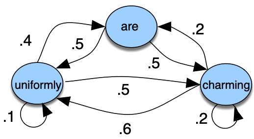
Observable Markov models
Example
States: {uniformly, are, charming}
Hidden phenomenon
Very often the things you observe in the real world can be thought of as a function of some other hidden variables.
Example 1:
Observations: Acoustic features of the speech signal, hidden states: phonemes that are spoken
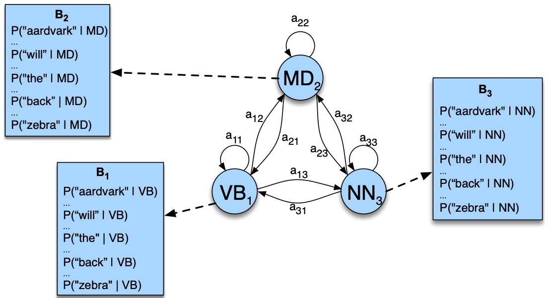
Example 2:
Observations: Words, hidden states: parts-of-speech
More examples
Observations: Encrypted symbols, hidden states: messages
Observations: Exchange rates, hidden states: volatility of the market
2. HMM definition and example#
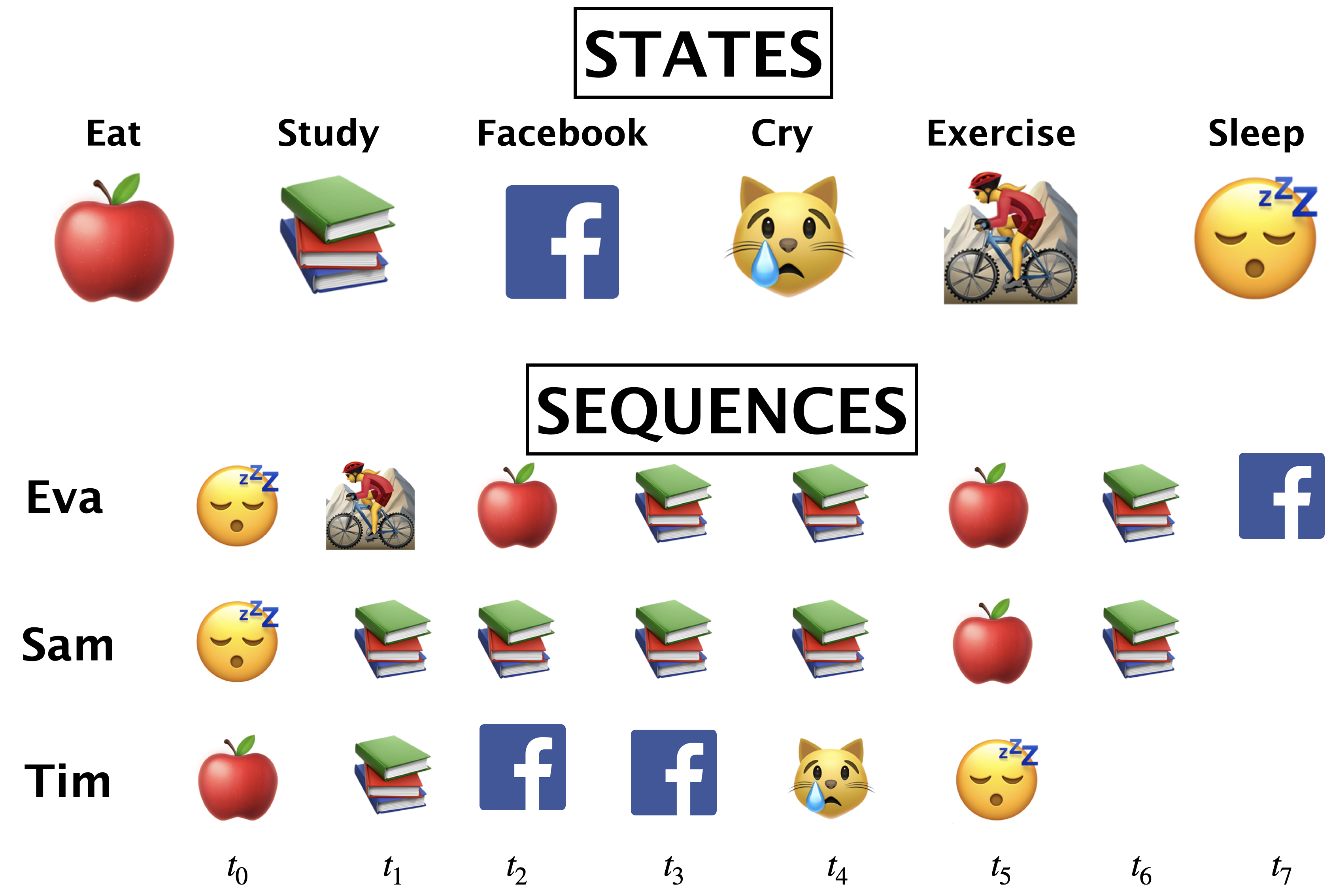
Last week we used the following toy example to demonstrate how do we learn initial state probabilities and transition probabilities in Markov models.
Imagine you’re developing a system for a company interested in tailoring its services based on users’ emotional states. (Though, remember, this is a simplified and hypothetical scenario to understand HMMs.)
In this scenario, the company cannot directly know a person’s emotional state because it’s ‘hidden’. However, they can observe behaviors through activity on their platform, like the types of videos watched or search queries.
2.1 Markov process with hidden variables: Example#
Let’s simplify the example above.
Suppose you have a little robot that is trying to estimate the posterior probability that you are Happy (H or 🙂) or Sad (S or 😔), given that the robot has observed whether you are doing one of the following activities:
Learning data science (L or 📚)
Eat (E or 🍎)
Cry (C or 😿)
Social media (F)
The robot is trying to estimate the unknown (hidden) state \(Q\), where \(Q =H\) when you are happy (🙂) and \(Q = S\) when you are sad (😔).
The robot is able to observe the activity you are doing: \(O = {L, E, C, F}\)
By observing activities, the goal is to infer the underlying emotional states (the hidden states) and understand the transition patterns between these states.
(Attribution: Example adapted from here.)
Example questions we are interested in answering are:
Given an HMM, what is the probability of observation sequence 📚📚😿📚📚? (this lecture)
Given an HMM, what is the best possible sequence of state of mind (e.g.,🙂,🙂,😔,🙂,🙂 ) given an observation sequence (e.g., L,L,C,L,L or 📚📚😿📚📚). (next lecture)
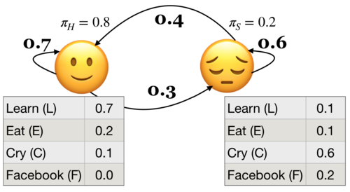
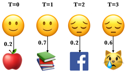
2.2 HMM ingredients#
State space (e.g., 🙂 (H), 😔 (S))
An initial probability distribution over the states
Transition probabilities
Emission probabilities
Conditional probabilities for all observations given a hidden state
Example: Below \(P(L|🙂) = 0.7\) and \(P(L|😔) = 0.1\)
Definition of an HMM
A hidden Markov model (HMM) is specified by the 5-tuple: \(\{S, Y, \pi, T, B\}\)
\(S = \{s_1, s_2, \dots, s_n\}\) is a set of states (e.g., moods)
\(Y = \{y_1, y_2, \dots, y_k\}\) is output alphabet (e.g., set of activities)
\(\pi = {\pi_1, \pi_2, \dots, \pi_n}\) is discrete initial state probability distribution
Transition probability matrix \(T\), where each \(a_{ij}\) represents the probability of moving from state \(s_i\) to state \(s_j\)
Emission probabilities $B = b_i(o), i \in S, o \in Y$
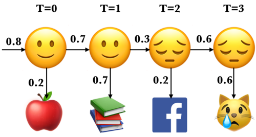
Yielding the state sequence and the observation sequences in an unrolled HMM
State sequence: \(Q = {q_0,q_1, q_2, \dots q_T}, q_i \in S\)
Observation sequence: \(O = {o_0,o_1, o_2, \dots o_T}, o_i \in Y\)
Here is an example of an unrolled HMM for six time steps, a possible realization of a sequence of states and a sequence of observations.
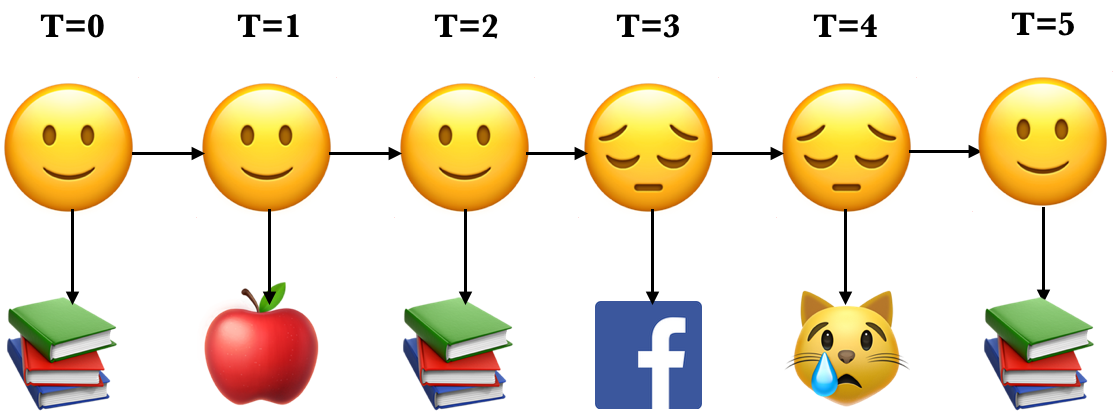
Each state produces only a single observation and the sequence of hidden states and the sequence of observations have the same length.
2.2 HMM assumptions#
The probability of a particular state only depends on the previous state.
\(P(q_i|q_0,q_1,\dots,q_{i-1})\) = \(P(q_i|q_{i-1})\)
The probability of an output observation \(o_i\) depends only on the state that produces the observation and not on any other state or any other observation.
\(P(o_i|q_0,q_1,\dots,q_{i}, o_0,o_1,\dots,o_{i-1})\) = \(P(o_i|q_i)\)
2.3 Three fundamental questions for an HMM#
Likelihood#
Given a model with parameters \(\theta = <\pi, T, B>\), how do we efficiently compute the likelihood of a particular observation sequence \(O\)?
Decoding#
Given an observation sequence \(O\) and a model \(\theta\) how do we choose a state sequence \(Q={q_0, q_1, \dots q_T}\) that best explains the observation sequence?
Learning#
Training: Given a large observation sequence \(O\) how do we choose the best parameters \(\theta\) that explain the data \(O\)?
❓❓ Questions for you#
Exercise 3.1: Select all of the following statements which are True (iClicker)#
(A) Emission probabilities in our toy example give us the probabilities of being happy or sad given that you are performing one of the four activities: Learn, Eat, Cry, Facebook.
(B) In hidden Markov models, the observation at time step \(t\) is conditionally independent of previous observations and previous hidden states given the hidden state at time \(t\).
(C) In hidden Markov models, given the hidden state at time \(t-1\), the hidden state at time step \(t\) is conditionally independent of the previous hidden states and observations.
(D) In hidden Markov models, each hidden state has a probability distribution over all observations.
Exercise 3.1: V’s Solutions!
B, C, D
Exercise 3.2: Discuss the following questions with your neighbour.#
What are the parameters \(\theta\) of a hidden Markov model?
Below is a hidden Markov model that relates numbers of ice creams eaten by Jason to the weather. Identify observations, hidden states, transition probabilities, and emission probabilities in the model.
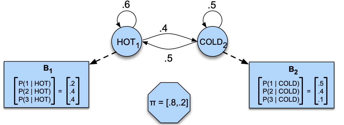
Exercise 3.2: V’s Solutions!
initial state probabilities \(\pi_0\), transition probabilities \(T\), emission probabilities \(B\)
Observations: 1, 2, 3
Hidden states: HOT, COLD
transition probabilities:
HOT |
COLD |
|
|---|---|---|
HOT |
0.6 |
0.4 |
COLD |
0.5 |
0.5 |
Emission probabilities:
1 |
2 |
3 |
|
|---|---|---|---|
HOT |
0.2 |
0.4 |
0.4 |
COLD |
0.5 |
0.4 |
0.1 |
Break (~5 mins)#

3. Likelihood#
In the context of HMMs, the likelihood of an observation sequence is the probability of observing that sequence given a particular set of model parameters \(\theta\).
Given a model with parameters \(\theta = <\pi, T, B>\), how do we efficiently compute the likelihood of a particular observation sequence \(O\)?
Example: What’s the probability of the sequence below?

Recall that in HMMs, the observations are dependent upon the hidden states in the same time step. Let’s consider a particular state sequence.
Probability of an observation sequence given the state sequence#
Suppose we know both the sequence of hidden states (moods) and the sequence of activities emitted by them.
\(P(O|Q) = \prod\limits_{i=1}^{T} P(o_i|q_i)\)
\(P(E L F C|🙂 🙂 😔 😔) = P(E|🙂) \times P(L|🙂) \times P(F|😔) \times P(C|😔)\)
3.1 Joint probability of observations and a possible hidden sequence#
Let’s consider the joint probability of being in a particular state sequence \(Q\) and generating a particular sequence \(O\) of activities.
\(P(O,Q) = P(O|Q)\times P(Q) = \prod\limits_{i=1}^T P(o_i|q_i) \times \prod\limits_{i=1}^T P(q_i|q_{i-1})\)
For example, for our toy sequence:
3.2 Total probability of an observation sequence#
But we do not know the hidden state sequence \(Q\).
We need to look at all combinations of hidden states.
We need to compute the probability of activity sequence (ELFC) by summing over all possible state (mood) sequences.
\(P(O) = \sum\limits_Q P(O,Q) = \sum\limits_QP(O|Q)P(Q)\)
Computationally inefficient
For HMMs with \(n\) hidden states and an observation sequence of \(T\) observations, there are \(n^T\) possible hidden sequences!!
In real-world problems, both \(n\) and \(T\) are large numbers.
How to compute \(P(O)\) cleverly?
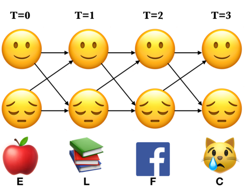
To avoid this complexity we use dynamic programming; we remember the results rather than recomputing them.
We make a trellis which is an array of states vs. time.
Note the alternative paths in the trellis. We are covering all the 16 combinations of states.
We compute \(\alpha_i(t)\), which represents the total probability of seeing the first \(t\) observations and ending up in state \(i\) at time \(t\), considering all possible paths that could have led there.
3.3 The forward procedure#
Intuition
To compute \(\alpha_j(t)\), we can compute \(\alpha_{i}(t-1)\) for all possible states \(i\) and then use our knowledge of \(a_{ij}\) and \(b_j(o_t)\).
We compute the trellis left-to-right because of the convention of time.
Remember that \(o_t\) is fixed and known.
Three steps of the forward procedure.
Initialization: Compute the \(\alpha\) values for nodes in the first column of the trellis \((t = 0)\).
Induction: Iteratively compute the \(\alpha\) values for nodes in the rest of the trellis \((1 \leq t < T)\).
Conclusion: Sum over the \(\alpha\) values for nodes in the last column of the trellis \((t = T)\).
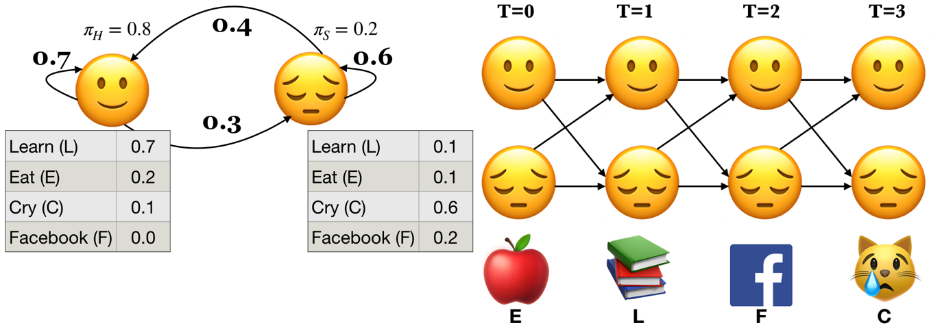
3.3.1 The forward procedure: Initialization \(\alpha_🙂(0)\) and \(\alpha_😔(0)\)#
Compute the nodes in the first column of the trellis \((T = 0)\).
Probability of starting at state 🙂 and observing the activity E: \(\alpha_🙂(0) = \pi_🙂 \times b_🙂(E) = 0.8 \times 0.2 = 0.16\)
Probability of starting at state 😔 and observing the activity E: \(\alpha_😔(0) = \pi_😔 \times b_😔(E) = 0.2 \times 0.1 = 0.02\)
3.3.2 The forward procedure: Induction#
Iteratively compute the nodes in the rest of the trellis \((1 \leq t < T)\).
To compute \(\alpha_j(t+1)\) we can compute \(\alpha_{i}(t)\) for all possible states \(i\) and then use our knowledge of \(a_{ij}\) and \(b_j(o_{t+1})\)
\(\alpha_j(t+1) = \sum\limits_{i=1}^n \alpha_i(t) a_{ij} b_j(o_{t+1})\)
The forward procedure: Induction \(\alpha_🙂(1)\)
\(\alpha_j(t+1) = \sum\limits_{i=1}^n \alpha_i(t) a_{ij} b_j(o_{t+1})\)
Probability of being at state 🙂 at \(t=1\) and observing the activity L
The forward procedure: Induction \(\alpha_😔(1)\)
\(\alpha_j(t+1) = \sum\limits_{i=1}^n \alpha_i(t) a_{ij} b_j(o_{t+1})\)
Probability of being at state 😔 at \(t=1\) and observing the activity L:
The forward procedure: Induction \(\alpha_🙂(2)\)
\(\alpha_j(t+1) = \sum\limits_{i=1}^n \alpha_i(t) a_{ij} b_j(o_{t+1})\)
Probability of being at state 🙂 at \(t=2\) and observing the activity F
The forward procedure: Induction \(\alpha_😔(2)\)
\(\alpha_j(t+1) = \sum\limits_{i=1}^n \alpha_i(t) a_{ij} b_j(o_{t+1})\)
Probability of being at state 😔 at \(t=2\) and observing the activity F:
The forward procedure: Induction \(\alpha_🙂(3)\)
\(\alpha_j(t+1) = \sum\limits_{i=1}^n \alpha_i(t) a_{ij} b_j(o_{t+1})\)
Probability of being at state 🙂 at \(t=3\) and observing the activity C:
The forward procedure: Induction \(\alpha_😔(3)\)
\(\alpha_j(t+1) = \sum\limits_{i=1}^n \alpha_i(t) a_{ij} b_j(o_{t+1})\)
Probability of being at state 😔 at \(t=3\) and observing the activity C:
3.3.3 The forward procedure: Conclusion#
Sum over all possible final states:
\(P(O;\theta) = \sum\limits_{i=1}^{n}\alpha_i(T-1)\)
\(P(E,L,F,C) = \alpha_🙂(3) + \alpha_😔(3) = 2.3 \times 10^{-4} + 2.07 \times 10^{-3}\)
Recap: The forward algorithm#
The forward algorithm computes likelihood of a given observation sequence: \(P(O;\theta)\).
For each state \(i\), we calculated \(\alpha_i(0), \alpha_i(1), \alpha_i(2), ...\alpha_i(t)\), which represent total probability of seeing the first \(t\) observations and ending up in state \(i\) at time \(t\), considering all possible paths that could have led there.
The trellis was computed left to right and top to bottom.
The forward algorithm stores the probabilities of all possible 1-state sequences (from the start), to store all possible 2-state sequences (from the start), to store all possible 3-state sequences (from the start) and so on.
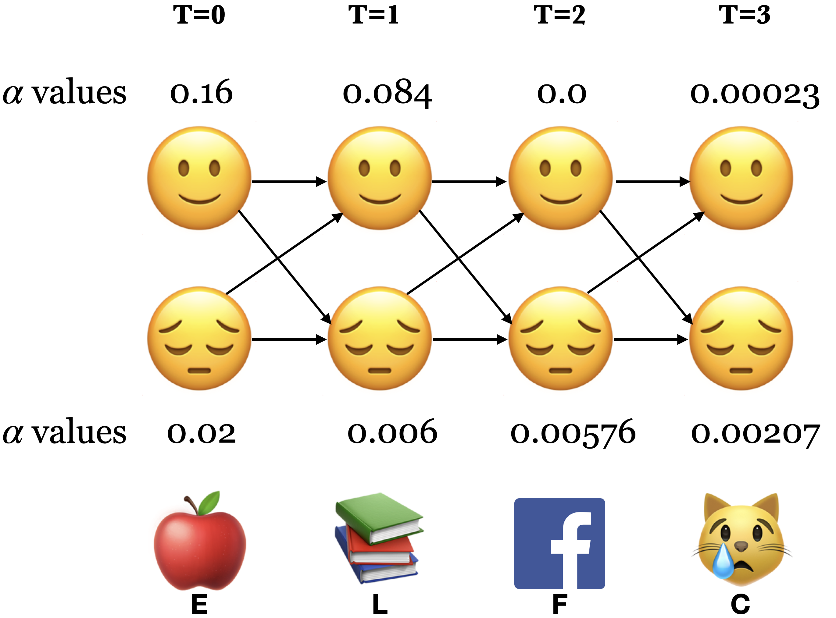
Sum over all possible final states:
\(P(O;\theta) = \sum\limits_{i=1}^{n}\alpha_i(T-1)\)
\(P(E,L,F,C) = \alpha_🙂(3) + \alpha_😔(3) = 0.00023 + 0.00207 = 0.0023\)
4. Supervised training of HMMs#
4.1 Supervised training of HMMs#
Suppose we have training data where we have \(O\) and corresponding \(Q\), then we can use MLE to learn parameters \(\theta = <\pi, T, B>\)
Get transition matrix and the emission probabilities.
Suppose \(i\), \(j\) are unique states from the state space and \(k\) is a unique observation.
\(\pi_0(i) = P(q_0 = i) = \frac{Count(q_0 = i)}{\#sequences}\)
\(a_{ij} = P(q_{t+1} = j|q_t = i) = \frac{Count(i,j)}{Count(i, anything)}\)
\(b_i(k) = P(o_{t} = k|q_t = i) = \frac{Count(i,k)}{Count(i, anything)}\)
Suppose we have training data where we have \(O\) and corresponding \(Q\), then we can use MLE to learn parameters \(\theta = <\pi, T, B>\)
Count how often \(q_{i-1}\) and \(q_i\) occur together normalized by how often \(q_{i-1}\) occurs with anything: \(p(q_i|q_{i-1}) = \frac{Count(q_{i-1} q_i)}{Count(q_{i-1} \text{anything})}\)
Count how often \(q_i\) is associated with the observation \(o_i\).
\(p(o_i|q_{i}) = \frac{Count(o_i \wedge q_i)}{Count(q_{i} \text{anything})}\)
In real life, all the calculations above are done with log probabilities for numerical stability.
4.2 HMM libraries#
Usually, practitioners develop there own version of HMMs suitable for their application. But there are some popular libraries:
Note that there are not many actively maintained off-the-shelf libraries available for supervised training of HMMs. seqlearn used to be part of
sklearn. But it’s separated now and is not being maintained.
Let’s calculate the likelihood of observing an observation sequence given a particular set of model parameters \(\theta\) using hmmlearn.
To run the code below successfully, you need install networkx and graphviz.
conda install -c conda-forge graphviz
conda install -c conda-forge python-graphviz
conda install -c anaconda networkx
conda install -c anaconda pydot
conda install --channel conda-forge pygraphviz
from hmmlearn import hmm

# Initializing an HMM
states = ["Happy", "Sad"]
n_states = len(states)

symbols = ["Learn", "Eat", "Cry", "Facebook"]
n_observations = len(symbols)

model = hmm.CategoricalHMM(
    n_components=n_states, random_state=42
)  # for discrete observations

# Set the initial state probabilities
model.startprob_ = np.array([0.8, 0.2])

# Set the transition matrix
model.transmat_ = np.array([[0.7, 0.3], [0.4, 0.6]])

# Set the emission probabilities of shape (n_components, n_symbols)
model.emissionprob_ = np.array([[0.7, 0.2, 0.1, 0.0], [0.1, 0.1, 0.6, 0.2]])
visualize_hmm(model, states=["happy", "sad"]) # user-defined function from code/plotting_functions.py
print("Emission probabilities: ")
pd.DataFrame(data=model.emissionprob_, columns=symbols, index=states)
We can calculate the probability of an observation sequence efficiently using the forward algorithm.
In
hmmlearn, we can use the.scoremethod of the hmm model to get the log probabilities.
obs_seq = np.array([[1], [0], [3], [2]])
label_obs_seq = map(lambda x: symbols[x], obs_seq.T[0])
# ?model.score
print(
    "Log likelihood of sequence %s is %s "
    % (list(label_obs_seq), model.score(obs_seq))
)
❓❓ Questions for you#
Exercise 3.2: Select all of the following statements which are True (iClicker)#
(A) In the forward algorithm we assume that the observation sequence \(O\) and the model parameters are fixed and known.
(B) In the forward algorithm, in our notation, \(\alpha_{i}(t)\) represents total probability of seeing the first \(t\) observations and ending up in state \(i\) at time \(t\), considering all possible paths that could have led there.
(C) In the forward algorithm \(\alpha_i(t)\) does not know anything about the future time steps after the time step \(t\).
(D) We conclude the forward procedure by summing over the \(\alpha\) values at the last time step.
(E) You can pass sequences of different lengths when training HMMs.
Exercise 3.2: V’s Solutions!
A, B, C, D, E
❓❓ Questions for you#
Exercise 3.3: Discuss the following question with your neighbour.#
The forward procedure using dynamic programming needs only \(\approx 2n^2T\) multiplications compared to the \(\approx(2T)n^T\) multiplications with the naive approach!! Why? Discuss with your neighbour.
Give an advantage of using the forward procedure compared to summing over all possible state combinations of length T.
Quick summary#
Summary#
Hidden Markov models (HMMs) model time-series with latent factors.
There are tons of applications associated with them and they are more realistic than Markov models.
The most successful application of HMMs is speech recognition.
Important ideas we learned#
HMM ingredients
Hidden states (e.g., Happy, Sad)
Output alphabet or output symbols (e.g., learn, study, cry, facebook)
Discrete initial state probability distribution
Transition probabilities
Emission probabilities
Fundamental questions for HMMs#
Three fundamental questions for HMMs:
likelihood
decoding
parameter learning
The forward algorithm is a dynamic programming algorithm to efficiently calculate the probability of an observation sequence given an HMM.
Supervised training of HMMs#
HMMs for POS tagging.
Not many tools out there for supervised training of HMMs.
Coming up#
Decoding: Viterbi algorithm
Given an HMM model and an observation sequence, how do we efficiently compute the corresponding hidden state sequence.
Unsupervised training of HMMs (Optional)
Resources#
Attribution: Many presentation ideas in this notebook are taken from Frank Rudzicz’s slides.