socceranalysisR

# install.packages("devtools")
# devtools::install_github("UBC-MDS/socceranalysisR")
# library(socceranalysisR)
# As out package is not published yet, use devtools::load_all() first 
devtools::load_all()
#> ℹ Loading socceranalysisR
#> 
#> Attaching package: 'dplyr'
#> 
#> 
#> The following objects are masked from 'package:stats':
#> 
#>     filter, lag
#> 
#> 
#> The following objects are masked from 'package:base':
#> 
#>     intersect, setdiff, setequal, union
#> 
#> 
#> ── Attaching packages ─────────────────────────────────────── tidyverse 1.3.2 ──
#> ✔ ggplot2 3.4.0     ✔ purrr   0.3.4
#> ✔ tibble  3.1.8     ✔ stringr 1.4.1
#> ✔ tidyr   1.2.0     ✔ forcats 0.5.2
#> ✔ readr   2.1.2     
#> ── Conflicts ────────────────────────────────────────── tidyverse_conflicts() ──
#> ✖ dplyr::filter() masks stats::filter()
#> ✖ dplyr::lag()    masks stats::lag()

Suppose you have three soccer data set:

small_data_1 <- data.frame(age = - c(18, 20, 20, 25, 25, 24, 25, 30, 33, 32, 44, 30, 17),
                         Wages_Euros = c(300000, 575000,    150000, 475000,375000,  225000, 225000, 200000, 225000, 250000, 250000, 375000, 200000))
small_data_2 <- data.frame (Name  = c("Flora", "Mary", "Sarah", "Ester", "Sophie", "Maria"),
second_column = c(1, 4, 3, 5, 1, 6),
third_column  = c(7, 30, 12, 17, 34,8))
 
small_data_3 <- data.frame(Team=  c("A", "B", "B", "B", "C", "C") ,
                       Market_Value_Euros = c(375000,   225000, 225000, 200000, 225000, 250000),
                       age = c(18, 20, 20, 25, 25, 24)) 

Generates meaningful visualizations to help users understand and interpret the numerical data using soc_viz_stats

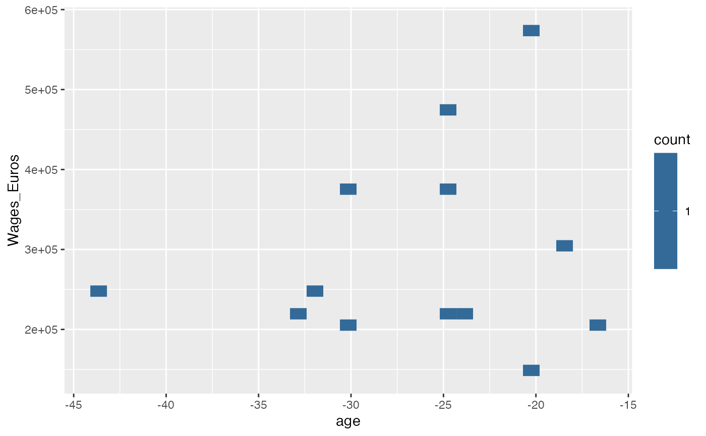
You can view any two chosen columns in a binned scatter plots by:

## scatter plots
soc_viz_stats('age', 'Wages_Euros', T , small_data_1)
#> Warning: `label_number_si()` was deprecated in scales 1.2.0.
#> ℹ Please use the `scale_cut` argument of `label_number()` instead.
#> ℹ The deprecated feature was likely used in the socceranalysisR package.
#>   Please report the issue to the authors.

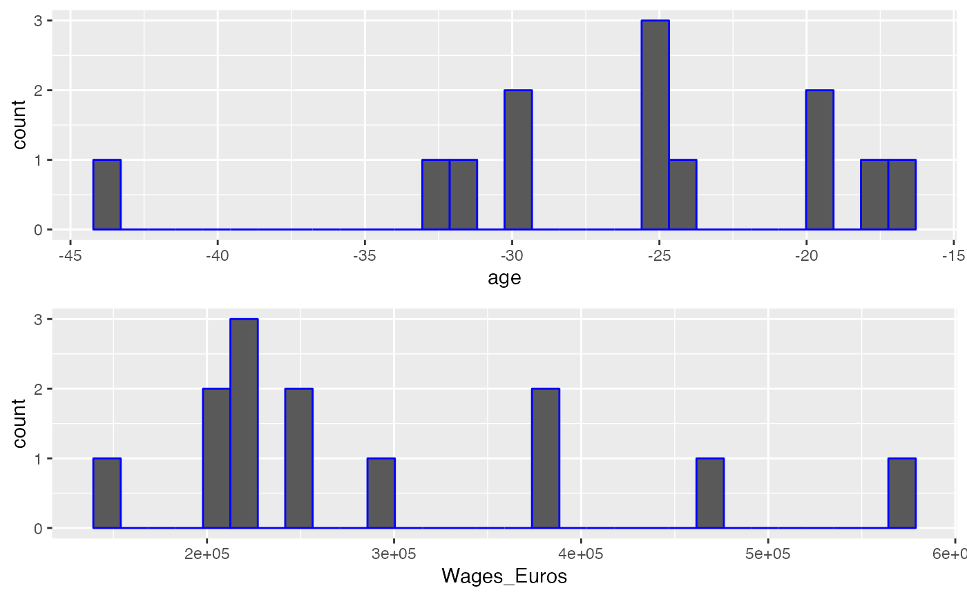
Or you can view the distribution them as two histograms:

## histograms
soc_viz_stats('age', 'Wages_Euros', FALSE , small_data_1)
#> `stat_bin()` using `bins = 30`. Pick better value with `binwidth`.
#> `stat_bin()` using `bins = 30`. Pick better value with `binwidth`.

Identifes outliers using statistical methods using soc_get_outliers

You can also get the outliers based on standard deviations methods:

## getting outliers
soc_get_outliers(small_data_1,Wages_Euros,"SD",2)
#>   age Wages_Euros
#> 1 -20      575000

Ranks players based on specific attributes with soc_rankingplayers

You can also rank players by their names based on the second feature by:

# ranking players 
rankingplayers(small_data_2, "second_column")
#>     Name second_column
#> 1  Maria             6
#> 2  Ester             5
#> 3   Mary             4
#> 4  Sarah             3
#> 5  Flora             1
#> 6 Sophie             1

provides a quick and easy way to understand the descriptive statistics of a team with soc_find_team_stat

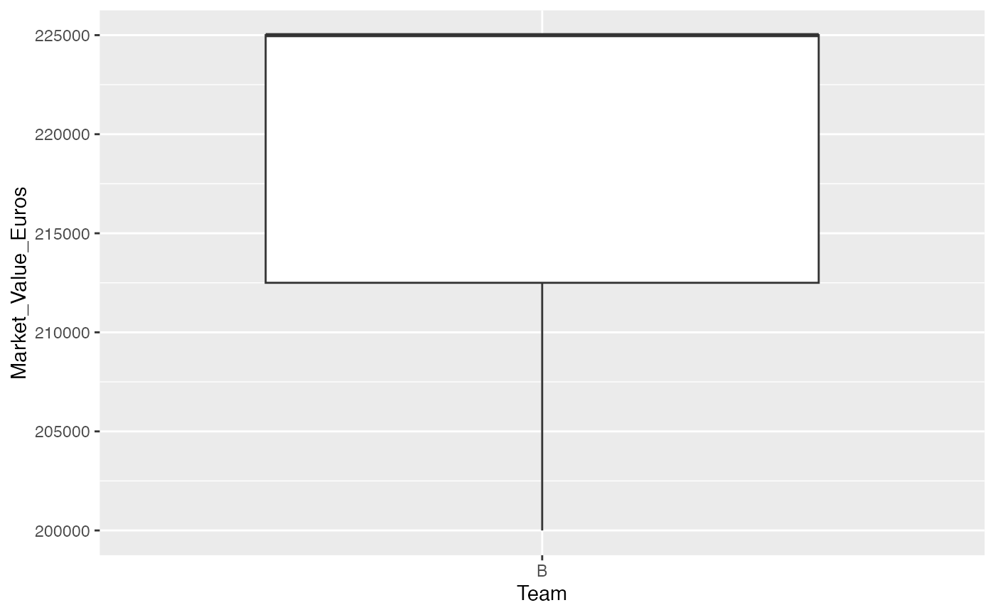
Finally, you can view a team’s descriptive statistics table and box-plot of selected feature:

# descriptive statistics
soc_find_team_stat(small_data_3, "B", Market_Value_Euros)
#> [[1]]
#>      Team           Market_Value_Euros      age       
#>  Length:3           Min.   :200000     Min.   :20.00  
#>  Class :character   1st Qu.:212500     1st Qu.:20.00  
#>  Mode  :character   Median :225000     Median :20.00  
#>                     Mean   :216667     Mean   :21.67  
#>                     3rd Qu.:225000     3rd Qu.:22.50  
#>                     Max.   :225000     Max.   :25.00  
#> 
#> [[2]]