C Heavy-Tailed Distributions
Consider the weekly returns of the Singapore Straights (STI) market, depicted by the following histogram. You’ll notice some extreme values that are far from the “bulk” of the data.
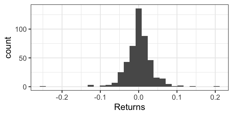
Traditional practice was to view these extremes as “outliers” that are a nuisance for analysis, and therefore should be removed. But this can actually be detrimental to the analysis, because these outliers are real occurences that should be anticipated.
Instead, Extreme Value Analysis is a practice that tries to get a sense of how big and how frequently extremes will happen.
C.1 Sensitivity of the mean to extremes
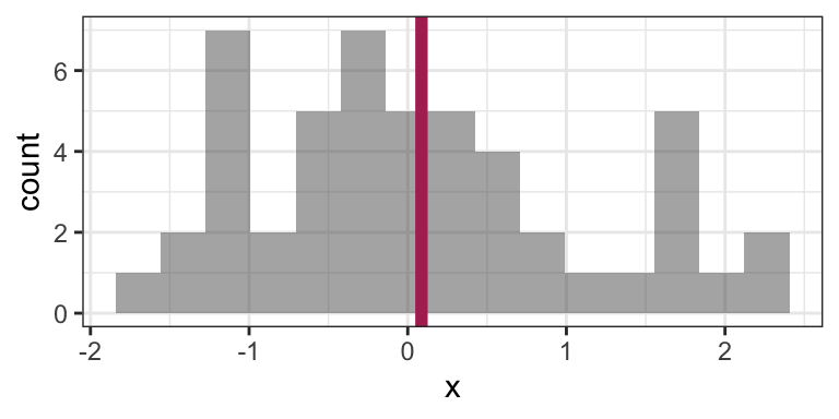
Indeed, the empirical (arithmetic) mean is sensitive to outliers: consider the sample average of 100 observations coming from a N(0,1) distribution:
set.seed(6)
n <- 50
x <- rnorm(n)
mean(x)
## [1] 0.08668773Here’s that mean depicted on a histogram of the data:
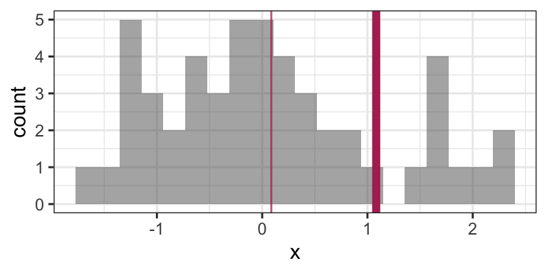
Now consider calculating the mean by replacing the last observation with 50 (a very large number):
x[n] <- 50
mean(x)
## [1] 1.082927This is a big difference made by a single observation! Let’s take a look at the histogram now (outlier not shown). The “old” mean is the thin vertical line:
There are robust and/or resistant ways of estimating the mean that are less sensitive to the outliers. But what’s more interesting when you have extreme values in your data is to get a sense of how frequently extremes will happen, and the mean won’t give you that sense.
C.2 Heavy-tailed Distributions
Distributions known as heavy-tailed distributions give rise to extreme values. These are distributions whose tail(s) decay like a power decay. The slower the decay, the heavier the tail is, and the more prone extreme values are.
For example, consider the member of the Pareto Type I family of distributions with survival function \(S(x) = 1/x\) for \(x \geq 1\). Here is this distribution compared to an Exponential(1) distribution (shifted to start at \(x=1\)):
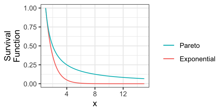
Notice that the Exponential survival function becomes essentially zero very quickly, whereas there’s still lots of probability well into the tail of the Pareto distribution.
Also note that if a distribution’s tail is “too heavy”, then its mean will not exist! For example, the above Pareto distribution has no mean.
C.3 Heavy-tailed distribution families
Here are some main families that include heavy-tailed distributions:
- Family of Generalized Pareto distributions
- Family of Generalized Extreme Value distributions
- Family of Student’s t distributions
- The Cauchy distribution is a special case of this.
C.4 Extreme Value Analysis
There are two key approaches in Extreme Value Analysis:
- Model the tail of a distribution using a theoretical model. That is, choose some
xvalue, and model the distribution beyond that point. It turns out a Generalized Pareto distribution is theoretically justified. - The peaks over thresholds method models the extreme observations occurring in a defined window of time. For example, the largest river flows each year. It turns out a Generalized Extreme Value distribution is theoretically justified here.
C.5 Multivariate Student’s t distributions
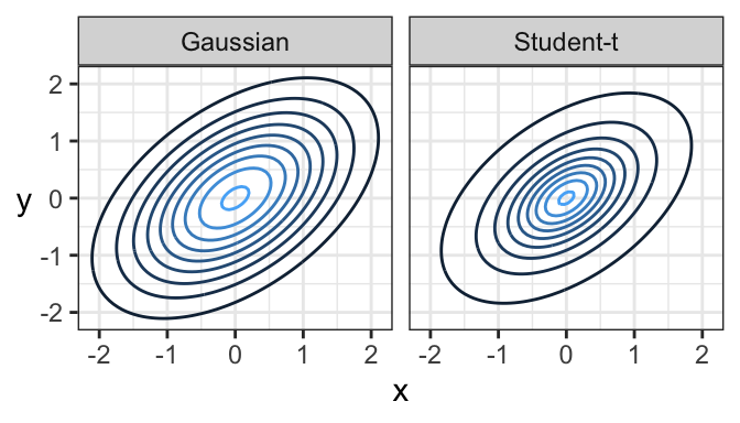
Just like there’s a multivariate Gaussian distribution, there’s also a multivariate Student’s t distribution. And in fact, its contours are elliptical, too!
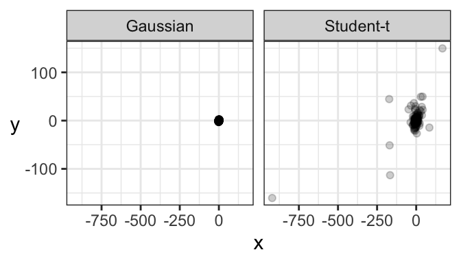
Here’s a comparison of a bivariate Gaussian and a bivariate Student’s t distribution, both of which are elliptical. One major difference is that a sample from a bivariate Gaussian distribution tends to be tightly packed, whereas data from a bivariate Student’s t distribution is prone to data deviating far from the main “data cloud”.
And here are samples coming from these two distributions. Notice how tightly bundled the Gaussian distribution is compared to the t distribution!