Lecture 4: Feature importances and feature selection

Lecture 4: Feature importances and feature selection#

UBC Master of Data Science program, 2022-23

Instructor: Varada Kolhatkar

Imports and LOs#

Imports#

import os
import string
import sys
from collections import deque

import matplotlib.pyplot as plt
import numpy as np
import pandas as pd

sys.path.append("code/.")
import seaborn as sns
from plotting_functions import *
from sklearn import datasets
from sklearn.compose import ColumnTransformer, make_column_transformer
from sklearn.dummy import DummyRegressor
from sklearn.ensemble import RandomForestRegressor
from sklearn.impute import SimpleImputer
from sklearn.linear_model import Ridge
from sklearn.model_selection import (
    cross_val_score,
    cross_validate,
    train_test_split,
)
from sklearn.pipeline import Pipeline, make_pipeline
from sklearn.preprocessing import OneHotEncoder, OrdinalEncoder, StandardScaler
from sklearn.svm import SVR
from utils import *

%matplotlib inline

Learning outcomes#

From this lecture, students are expected to be able to:

Explain the limitations of simple correlation-based approaches to identify feature importances.
Interpret the coefficients of linear regression, including for scaled numeric features.
Explain the purpose of feature selection.
Discuss and compare different feature selection methods at a high level.
Explain and use model-based feature selection.
Explain recursive feature elimination at a high level.
Use sklearn’s implementation of recursive feature elimination (RFE).
Explain how RFECV (cross-validated recursive feature elimination) works.
Explain forward and backward feature selection at a high level.
Use sklearn’s implementation of forward and backward selection.

I’m using seaborn in this lecture for easy heatmap plotting, which is not in the course environment. You can install it as follows.

> conda activate 573
> conda install -c anaconda seaborn

import warnings

warnings.simplefilter(action="ignore", category=FutureWarning)

Data#

In the first part of this lecture, we’ll be using Kaggle House Prices dataset, the dataset we used in lecture 10. As usual, to run this notebook you’ll need to download the data. Unzip the data into a subdirectory called data. For this dataset, train and test have already been separated. We’ll be working with the train portion in this lecture.

df = pd.read_csv("data/housing-kaggle/train.csv")
train_df, test_df = train_test_split(df, test_size=0.10, random_state=123)
train_df.head()

	Id	MSSubClass	MSZoning	LotFrontage	LotArea	Street	Alley	LotShape	LandContour	Utilities	...	PoolQC	Fence	MiscFeature	MiscVal	MoSold	YrSold	SaleType	SaleCondition	SalePrice
302	303	20	RL	118.0	13704	Pave	NaN	IR1	Lvl	AllPub	...	NaN	NaN	NaN	0	1	2006	WD	Normal	205000
767	768	50	RL	75.0	12508	Pave	NaN	IR1	Lvl	AllPub	...	NaN	NaN	Shed	1300	7	2008	WD	Normal	160000
429	430	20	RL	130.0	11457	Pave	NaN	IR1	Lvl	AllPub	...	NaN	NaN	NaN	0	3	2009	WD	Normal	175000
1139	1140	30	RL	98.0	8731	Pave	NaN	IR1	Lvl	AllPub	...	NaN	NaN	NaN	0	5	2007	WD	Normal	144000
558	559	60	RL	57.0	21872	Pave	NaN	IR2	HLS	AllPub	...	NaN	NaN	NaN	0	8	2008	WD	Normal	175000

5 rows × 81 columns

The prediction task is predicting SalePrice given features related to properties.
Note that the target is numeric, not categorical.

train_df.shape

(1314, 81)

Let’s separate `X` and `y`#

X_train = train_df.drop(columns=["SalePrice"])
y_train = train_df["SalePrice"]

X_test = test_df.drop(columns=["SalePrice"])
y_test = test_df["SalePrice"]

Let’s identify feature types#

drop_features = ["Id"]
numeric_features = [
    "BedroomAbvGr",
    "KitchenAbvGr",
    "LotFrontage",
    "LotArea",
    "OverallQual",
    "OverallCond",
    "YearBuilt",
    "YearRemodAdd",
    "MasVnrArea",
    "BsmtFinSF1",
    "BsmtFinSF2",
    "BsmtUnfSF",
    "TotalBsmtSF",
    "1stFlrSF",
    "2ndFlrSF",
    "LowQualFinSF",
    "GrLivArea",
    "BsmtFullBath",
    "BsmtHalfBath",
    "FullBath",
    "HalfBath",
    "TotRmsAbvGrd",
    "Fireplaces",
    "GarageYrBlt",
    "GarageCars",
    "GarageArea",
    "WoodDeckSF",
    "OpenPorchSF",
    "EnclosedPorch",
    "3SsnPorch",
    "ScreenPorch",
    "PoolArea",
    "MiscVal",
    "YrSold",
]

ordinal_features_reg = [
    "ExterQual",
    "ExterCond",
    "BsmtQual",
    "BsmtCond",
    "HeatingQC",
    "KitchenQual",
    "FireplaceQu",
    "GarageQual",
    "GarageCond",
    "PoolQC",
]
ordering = [
    "Po",
    "Fa",
    "TA",
    "Gd",
    "Ex",
]  # if N/A it will just impute something, per below
ordering_ordinal_reg = [ordering] * len(ordinal_features_reg)
ordering_ordinal_reg

[['Po', 'Fa', 'TA', 'Gd', 'Ex'],
 ['Po', 'Fa', 'TA', 'Gd', 'Ex'],
 ['Po', 'Fa', 'TA', 'Gd', 'Ex'],
 ['Po', 'Fa', 'TA', 'Gd', 'Ex'],
 ['Po', 'Fa', 'TA', 'Gd', 'Ex'],
 ['Po', 'Fa', 'TA', 'Gd', 'Ex'],
 ['Po', 'Fa', 'TA', 'Gd', 'Ex'],
 ['Po', 'Fa', 'TA', 'Gd', 'Ex'],
 ['Po', 'Fa', 'TA', 'Gd', 'Ex'],
 ['Po', 'Fa', 'TA', 'Gd', 'Ex']]

ordinal_features_oth = [
    "BsmtExposure",
    "BsmtFinType1",
    "BsmtFinType2",
    "Functional",
    "Fence",
]
ordering_ordinal_oth = [
    ["NA", "No", "Mn", "Av", "Gd"],
    ["NA", "Unf", "LwQ", "Rec", "BLQ", "ALQ", "GLQ"],
    ["NA", "Unf", "LwQ", "Rec", "BLQ", "ALQ", "GLQ"],
    ["Sal", "Sev", "Maj2", "Maj1", "Mod", "Min2", "Min1", "Typ"],
    ["NA", "MnWw", "GdWo", "MnPrv", "GdPrv"],
]

categorical_features = list(
    set(X_train.columns)
    - set(numeric_features)
    - set(ordinal_features_reg)
    - set(ordinal_features_oth)
    - set(drop_features)
)
categorical_features

['LotConfig',
 'Alley',
 'MiscFeature',
 'LotShape',
 'RoofStyle',
 'Electrical',
 'Foundation',
 'RoofMatl',
 'Exterior2nd',
 'Exterior1st',
 'LandContour',
 'Utilities',
 'MasVnrType',
 'SaleCondition',
 'CentralAir',
 'MoSold',
 'Condition2',
 'BldgType',
 'GarageType',
 'GarageFinish',
 'LandSlope',
 'HouseStyle',
 'MSZoning',
 'Condition1',
 'Neighborhood',
 'MSSubClass',
 'PavedDrive',
 'Street',
 'Heating',
 'SaleType']

from sklearn.compose import ColumnTransformer, make_column_transformer

numeric_transformer = make_pipeline(SimpleImputer(strategy="median"), StandardScaler())
ordinal_transformer_reg = make_pipeline(
    SimpleImputer(strategy="most_frequent"),
    OrdinalEncoder(categories=ordering_ordinal_reg),
)

ordinal_transformer_oth = make_pipeline(
    SimpleImputer(strategy="most_frequent"),
    OrdinalEncoder(categories=ordering_ordinal_oth),
)

categorical_transformer = make_pipeline(
    SimpleImputer(strategy="constant", fill_value="missing"),
    OneHotEncoder(handle_unknown="ignore", sparse=False),
)

preprocessor = make_column_transformer(
    ("drop", drop_features),
    (numeric_transformer, numeric_features),
    (ordinal_transformer_reg, ordinal_features_reg),
    (ordinal_transformer_oth, ordinal_features_oth),
    (categorical_transformer, categorical_features),
)

preprocessor.fit(X_train)
preprocessor.named_transformers_

{'drop': 'drop',
 'pipeline-1': Pipeline(steps=[('simpleimputer', SimpleImputer(strategy='median')),
                 ('standardscaler', StandardScaler())]),
 'pipeline-2': Pipeline(steps=[('simpleimputer', SimpleImputer(strategy='most_frequent')),
                 ('ordinalencoder',
                  OrdinalEncoder(categories=[['Po', 'Fa', 'TA', 'Gd', 'Ex'],
                                             ['Po', 'Fa', 'TA', 'Gd', 'Ex'],
                                             ['Po', 'Fa', 'TA', 'Gd', 'Ex'],
                                             ['Po', 'Fa', 'TA', 'Gd', 'Ex'],
                                             ['Po', 'Fa', 'TA', 'Gd', 'Ex'],
                                             ['Po', 'Fa', 'TA', 'Gd', 'Ex'],
                                             ['Po', 'Fa', 'TA', 'Gd', 'Ex'],
                                             ['Po', 'Fa', 'TA', 'Gd', 'Ex'],
                                             ['Po', 'Fa', 'TA', 'Gd', 'Ex'],
                                             ['Po', 'Fa', 'TA', 'Gd', 'Ex']]))]),
 'pipeline-3': Pipeline(steps=[('simpleimputer', SimpleImputer(strategy='most_frequent')),
                 ('ordinalencoder',
                  OrdinalEncoder(categories=[['NA', 'No', 'Mn', 'Av', 'Gd'],
                                             ['NA', 'Unf', 'LwQ', 'Rec', 'BLQ',
                                              'ALQ', 'GLQ'],
                                             ['NA', 'Unf', 'LwQ', 'Rec', 'BLQ',
                                              'ALQ', 'GLQ'],
                                             ['Sal', 'Sev', 'Maj2', 'Maj1',
                                              'Mod', 'Min2', 'Min1', 'Typ'],
                                             ['NA', 'MnWw', 'GdWo', 'MnPrv',
                                              'GdPrv']]))]),
 'pipeline-4': Pipeline(steps=[('simpleimputer',
                  SimpleImputer(fill_value='missing', strategy='constant')),
                 ('onehotencoder',
                  OneHotEncoder(handle_unknown='ignore', sparse=False))])}

ohe_columns = list(
    preprocessor.named_transformers_["pipeline-4"]
    .named_steps["onehotencoder"]
    .get_feature_names(categorical_features)
)
new_columns = (
    numeric_features + ordinal_features_reg + ordinal_features_oth + ohe_columns
)

X_train_enc = pd.DataFrame(
    preprocessor.transform(X_train), index=X_train.index, columns=new_columns
)
X_train_enc

	BedroomAbvGr	KitchenAbvGr	LotFrontage	LotArea	OverallQual	OverallCond	YearBuilt	YearRemodAdd	MasVnrArea	BsmtFinSF1	...	Heating_Wall	SaleType_COD	SaleType_CWD	SaleType_Con	SaleType_ConLD	SaleType_ConLI	SaleType_ConLw	SaleType_New	SaleType_Oth	SaleType_WD
302	0.154795	-0.222647	2.312501	0.381428	0.663680	-0.512408	0.993969	0.840492	0.269972	-0.961498	...	0.0	0.0	0.0	0.0	0.0	0.0	0.0	0.0	0.0	1.0
767	1.372763	-0.222647	0.260890	0.248457	-0.054669	1.285467	-1.026793	0.016525	-0.573129	0.476092	...	0.0	0.0	0.0	0.0	0.0	0.0	0.0	0.0	0.0	1.0
429	0.154795	-0.222647	2.885044	0.131607	-0.054669	-0.512408	0.563314	0.161931	-0.573129	1.227559	...	0.0	0.0	0.0	0.0	0.0	0.0	0.0	0.0	0.0	1.0
1139	0.154795	-0.222647	1.358264	-0.171468	-0.773017	-0.512408	-1.689338	-1.679877	-0.573129	0.443419	...	0.0	0.0	0.0	0.0	0.0	0.0	0.0	0.0	0.0	1.0
558	0.154795	-0.222647	-0.597924	1.289541	0.663680	-0.512408	0.828332	0.598149	-0.573129	0.354114	...	0.0	0.0	0.0	0.0	0.0	0.0	0.0	0.0	0.0	1.0
...	...	...	...	...	...	...	...	...	...	...	...	...	...	...	...	...	...	...	...	...	...
1041	1.372763	-0.222647	-0.025381	-0.127107	-0.054669	2.184405	-0.165485	0.743555	0.843281	-0.090231	...	0.0	0.0	0.0	0.0	0.0	0.0	0.0	0.0	0.0	1.0
1122	0.154795	-0.222647	-0.025381	-0.149788	-1.491366	-2.310284	-0.496757	-1.389065	-0.573129	-0.961498	...	0.0	1.0	0.0	0.0	0.0	0.0	0.0	0.0	0.0	0.0
1346	0.154795	-0.222647	-0.025381	1.168244	0.663680	1.285467	-0.099230	0.888961	-0.573129	-0.314582	...	0.0	0.0	0.0	0.0	0.0	0.0	0.0	0.0	0.0	1.0
1406	-1.063173	-0.222647	0.022331	-0.203265	-0.773017	1.285467	0.033279	1.082835	-0.573129	0.467379	...	0.0	0.0	0.0	0.0	0.0	0.0	0.0	0.0	0.0	1.0
1389	0.154795	-0.222647	-0.454788	-0.475099	-0.054669	0.386530	-0.993666	-1.679877	-0.573129	-0.144686	...	0.0	0.0	0.0	0.0	0.0	0.0	0.0	0.0	0.0	1.0

1314 rows × 263 columns

X_train_enc.shape

(1314, 263)

lr_pipe = make_pipeline(preprocessor, Ridge())
scores = cross_validate(lr_pipe, X_train, y_train, return_train_score=True)
pd.DataFrame(scores)

	fit_time	score_time	test_score	train_score
0	0.037688	0.006314	0.834450	0.916827
1	0.033185	0.006056	0.810031	0.919218
2	0.018007	0.004891	0.831653	0.912397
3	0.020183	0.004715	0.843537	0.914043
4	0.017457	0.004584	0.548802	0.920476

Feature importances#

How does the output depend upon the input?
How do the predictions change as a function of a particular feature?
If the model is bad interpretability does not make sense.

SimpleFeature correlations#

Let’s look at the correlations between various features with other features and the target in our encoded data (first row/column).
In simple terms here is how you can interpret correlations between two variables $X$ and $Y$:
- If $Y$ goes up when $X$ goes up, we say $X$ and $Y$ are positively correlated.
- If $Y$ goes down when $X$ goes up, we say $X$ and $Y$ are negatively correlated.
- If $Y$ is unchanged when $X$ changes, we say $X$ and $Y$ are uncorrelated.

Let’s examine the correlations among different columns, including the target column.

cor = pd.concat((y_train, X_train_enc), axis=1).iloc[:, :10].corr()
plt.figure(figsize=(8, 6))
sns.set(font_scale=0.8)
sns.heatmap(cor, annot=True, cmap=plt.cm.Blues);

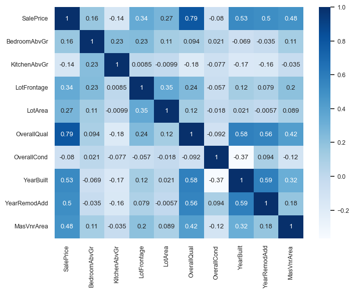
../_images/1fc3bc3cb57fc9d801a8fb3ad2bee1d82fc785a6e3bc3dadf666886eb9448a7f.png

We can immediately see that SalePrice is highly correlated with OverallQual.
This is an early hint that OverallQual is a useful feature in predicting SalePrice.
However, this approach is extremely simplistic.
- It only looks at each feature in isolation.
- It only looks at linear associations:
  - What if SalePrice is high when BsmtFullBath is 2 or 3, but low when it’s 0, 1, or 4? They might seem uncorrelated.

cor = pd.concat((y_train, X_train_enc), axis=1).iloc[:, 10:15].corr()
plt.figure(figsize=(4, 4))
sns.set(font_scale=0.8)
sns.heatmap(cor, annot=True, cmap=plt.cm.Blues);

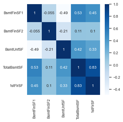
../_images/cbd338ffcd59a4835c102abc0ab44221ba4b31477058a22a38289c4aa6f76ec9.png

Looking at this diagram also tells us the relationship between features.
- For example, 1stFlrSF and TotalBsmtSF are highly correlated.
- Do we need both of them?
- If our model says 1stFlrSF is very important and TotalBsmtSF is very unimportant, do we trust those values?
- Maybe TotalBsmtSF only “becomes important” if 1stFlrSF is removed.
- Sometimes the opposite happens: a feature only becomes important if another feature is added.

Feature importances in linear models#

With linear regression we can look at the coefficients for each feature.
Overall idea: predicted price = intercept + $\sum_i$ coefficient i $\times$ feature i.

lr = make_pipeline(preprocessor, Ridge())
lr.fit(X_train, y_train);

Let’s look at the coefficients.

lr_coefs = pd.DataFrame(
    data=lr.named_steps["ridge"].coef_, index=new_columns, columns=["Coefficient"]
)
lr_coefs.head(20)

	Coefficient
BedroomAbvGr	-3723.741570
KitchenAbvGr	-4580.204576
LotFrontage	-1578.664421
LotArea	5109.356718
OverallQual	12487.561839
OverallCond	4855.535334
YearBuilt	4226.684842
YearRemodAdd	324.664715
MasVnrArea	5251.325210
BsmtFinSF1	3667.172851
BsmtFinSF2	583.114880
BsmtUnfSF	-1266.614671
TotalBsmtSF	2751.084018
1stFlrSF	6736.788904
2ndFlrSF	13409.901084
LowQualFinSF	-448.424132
GrLivArea	15988.182407
BsmtFullBath	2299.227266
BsmtHalfBath	500.169112
FullBath	2831.811467

Let’s try to interpret coefficients for different types of features.

Ordinal features#

The ordinal features are easiest to interpret.

print(ordinal_features_reg)

['ExterQual', 'ExterCond', 'BsmtQual', 'BsmtCond', 'HeatingQC', 'KitchenQual', 'FireplaceQu', 'GarageQual', 'GarageCond', 'PoolQC']

lr_coefs.loc["ExterQual"]

Coefficient    4195.671512
Name: ExterQual, dtype: float64

Increasing by one category of exterior quality (e.g. good -> excellent) increases the predicted price by $\sim\$4195$.
- Wow, that’s a lot!
- Remember this is just what the model has learned. It doesn’t tell us how the world works.

one_example = X_test[:1]

one_example[["ExterQual"]]

	ExterQual
147	Gd

Let’s perturb the example and change ExterQual to Ex.

one_example_perturbed = one_example.copy()
one_example_perturbed["ExterQual"] = "Ex"  # Change Gd to Ex

one_example_perturbed[["ExterQual"]]

	ExterQual
147	Ex

How does the prediction change after changing ExterQual from Gd to Ex?

print("Prediction on the original example: ", lr.predict(one_example))
print("Prediction on the perturbed example: ", lr.predict(one_example_perturbed))
print(
    "After changing ExterQual from Gd to Ex increased the prediction by: ",
    lr.predict(one_example_perturbed) - lr.predict(one_example),
)

Prediction on the original example:  [224795.63596803]
Prediction on the perturbed example:  [228991.30748049]
After changing ExterQual from Gd to Ex increased the prediction by:  [4195.67151247]

That’s exactly the learned coefficient for ExterQual!

lr_coefs.loc["ExterQual"]

Coefficient    4195.671512
Name: ExterQual, dtype: float64

So our interpretation is correct!

Increasing by one category of exterior quality (e.g. good -> excellent) increases the predicted price by $\sim\$4195$.

Categorical features#

What about the categorical features?
We have created a number of columns for each category with OHE and each category gets it’s own coefficient.

print(categorical_features)

['LotConfig', 'Alley', 'MiscFeature', 'LotShape', 'RoofStyle', 'Electrical', 'Foundation', 'RoofMatl', 'Exterior2nd', 'Exterior1st', 'LandContour', 'Utilities', 'MasVnrType', 'SaleCondition', 'CentralAir', 'MoSold', 'Condition2', 'BldgType', 'GarageType', 'GarageFinish', 'LandSlope', 'HouseStyle', 'MSZoning', 'Condition1', 'Neighborhood', 'MSSubClass', 'PavedDrive', 'Street', 'Heating', 'SaleType']

lr_coefs_landslope = lr_coefs[lr_coefs.index.str.startswith("LandSlope")]
lr_coefs_landslope

	Coefficient
LandSlope_Gtl	457.197456
LandSlope_Mod	7420.208381
LandSlope_Sev	-7877.405837

We can talk about switching from one of these categories to another by picking a “reference” category:

lr_coefs_landslope - lr_coefs_landslope.loc["LandSlope_Gtl"]

	Coefficient
LandSlope_Gtl	0.000000
LandSlope_Mod	6963.010925
LandSlope_Sev	-8334.603292

If you change the category from LandSlope_Gtl to LandSlope_Mod the prediction price goes up by $\sim\$6963$
If you change the category from LandSlope_Gtl to LandSlope_Sev the prediction price goes down by $\sim\$8334$

Note that this might not make sense in the real world but this is what our model decided to learn given this small amount of data.

one_example = X_test[:1]
one_example[['LandSlope']]

	LandSlope
147	Gtl

Let’s perturb the example and change LandSlope to Mod.

one_example_perturbed = one_example.copy()
one_example_perturbed["LandSlope"] = "Mod"  # Change Gd to Ex

one_example_perturbed[["LandSlope"]]

	LandSlope
147	Mod

How does the prediction change after changing LandSlope from Gtl to Mod?

print("Prediction on the original example: ", lr.predict(one_example))
print("Prediction on the perturbed example: ", lr.predict(one_example_perturbed))
print(
    "After changing ExterQual from Gd to Ex increased the prediction by: ",
    lr.predict(one_example_perturbed) - lr.predict(one_example),
)

Prediction on the original example:  [224795.63596803]
Prediction on the perturbed example:  [231758.64689313]
After changing ExterQual from Gd to Ex increased the prediction by:  [6963.0109251]

Our interpretation above is correct!

lr_coefs.sort_values(by="Coefficient")

	Coefficient
RoofMatl_ClyTile	-191129.774314
Condition2_PosN	-105552.840565
Heating_OthW	-27260.681308
MSZoning_C (all)	-21990.746193
Exterior1st_ImStucc	-19393.964621
...	...
PoolQC	34217.656047
RoofMatl_CompShg	36525.980874
Neighborhood_NridgHt	37532.643270
Neighborhood_StoneBr	39993.978324
RoofMatl_WdShngl	83646.711008

263 rows × 1 columns

For example, the above coefficient says that “If the roof is made of clay or tile, the predicted price is \$191K less”?
Do we believe these interpretations??
- Do we believe this is how the predictions are being computed? Yes.
- Do we believe that this is how the world works? No.

Note

If you did drop='first' (we didn’t) then you already have a reference class, and all the values are with respect to that one. The interpretation depends on whether we did drop='first', hence the hassle.

Interpreting coefficients of numeric features#

Let’s look at coefficients of PoolArea, LotFrontage, LotArea.

lr_coefs.loc[["PoolArea", "LotFrontage", "LotArea"]]

	Coefficient
PoolArea	2822.370476
LotFrontage	-1578.664421
LotArea	5109.356718

Intuition:

Tricky because numeric features are scaled!
Increasing PoolArea by 1 scaled unit increases the predicted price by $\sim\$2822$.
Increasing LotArea by 1 scaled unit increases the predicted price by $\sim\$5109$.
Increasing LotFrontage by 1 scaled unit decreases the predicted price by $\sim\$1578$.

Does that sound reasonable?

For PoolArea and LotArea, yes.
For LotFrontage, that’s surprising. Something positive would have made more sense?

It might be the case that LotFrontage is correlated with some other variable, which might have a larger positive coefficient.

BTW, let’s make sure the predictions behave as expected:

Example showing how can we interpret coefficients of scaled features.#

What’s one scaled unit for LotArea?
The scaler subtracted the mean and divided by the standard deviation.
The division actually changed the scale!
For the unit conversion, we don’t care about the subtraction, but only the scaling.

scaler = preprocessor.named_transformers_["pipeline-1"]["standardscaler"]

lr_scales = pd.DataFrame(
    data=np.sqrt(scaler.var_), index=numeric_features, columns=["Scale"]
)
lr_scales.head()

	Scale
BedroomAbvGr	0.821040
KitchenAbvGr	0.218760
LotFrontage	20.959139
LotArea	8994.471032
OverallQual	1.392082

It seems like LotArea was divided by 8994.471032 sqft.

lr_coefs.loc[["LotArea"]]

	Coefficient
LotArea	5109.356718

The coefficient tells us that if we increase the scaled LotArea by one scaled unit the price would go up by $\approx\$5109$.
One scaled unit represents $\sim 8994$ sqft in the original scale.

Let’s examine whether this behaves as expected.

X_test_enc = pd.DataFrame(
    preprocessor.transform(X_test), index=X_test.index, columns=new_columns
)

one_ex_preprocessed = X_test_enc[:1]
one_ex_preprocessed

	BedroomAbvGr	KitchenAbvGr	LotFrontage	LotArea	OverallQual	OverallCond	YearBuilt	YearRemodAdd	MasVnrArea	BsmtFinSF1	...	Heating_Wall	SaleType_COD	SaleType_CWD	SaleType_Con	SaleType_ConLD	SaleType_ConLI	SaleType_ConLw	SaleType_New	SaleType_Oth	SaleType_WD
147	0.154795	-0.222647	-0.025381	-0.085415	0.66368	-0.512408	0.993969	0.792023	0.438592	-0.961498	...	0.0	0.0	0.0	0.0	0.0	0.0	0.0	0.0	0.0	1.0

1 rows × 263 columns

orig_pred = lr.named_steps["ridge"].predict(one_ex_preprocessed)
orig_pred

/Users/kvarada/opt/miniconda3/envs/573/lib/python3.10/site-packages/sklearn/base.py:443: UserWarning: X has feature names, but Ridge was fitted without feature names
  warnings.warn(

array([224795.63596803])

one_ex_preprocessed_perturbed = one_ex_preprocessed.copy()
one_ex_preprocessed_perturbed["LotArea"] += 1  # we are adding one to the scaled LotArea
one_ex_preprocessed_perturbed

	BedroomAbvGr	KitchenAbvGr	LotFrontage	LotArea	OverallQual	OverallCond	YearBuilt	YearRemodAdd	MasVnrArea	BsmtFinSF1	...	Heating_Wall	SaleType_COD	SaleType_CWD	SaleType_Con	SaleType_ConLD	SaleType_ConLI	SaleType_ConLw	SaleType_New	SaleType_Oth	SaleType_WD
147	0.154795	-0.222647	-0.025381	0.914585	0.66368	-0.512408	0.993969	0.792023	0.438592	-0.961498	...	0.0	0.0	0.0	0.0	0.0	0.0	0.0	0.0	0.0	1.0

1 rows × 263 columns

We are expecting an increase of $5109.35671809 in the prediction compared to the original value of LotArea.

perturbed_pred = lr.named_steps["ridge"].predict(one_ex_preprocessed_perturbed)

/Users/kvarada/opt/miniconda3/envs/573/lib/python3.10/site-packages/sklearn/base.py:443: UserWarning: X has feature names, but Ridge was fitted without feature names
  warnings.warn(

perturbed_pred - orig_pred

array([5109.35671809])

Our interpretation is correct!

Humans find it easier to think about features in their original scale.
How can we interpret this coefficient in the original scale?
If I increase original LotArea by one square foot then the predicted price would go up by this amount:

5109.356718094072 / 8994.471032 # Coefficient learned on the scaled features / the scaling factor for this feature

0.5680552752814816

one_example = X_test[:1]

one_example

	Id	MSSubClass	MSZoning	LotFrontage	LotArea	Street	Alley	LotShape	LandContour	Utilities	...	ScreenPorch	PoolArea	PoolQC	Fence	MiscFeature	MiscVal	MoSold	YrSold	SaleType	SaleCondition
147	148	60	RL	NaN	9505	Pave	NaN	IR1	Lvl	AllPub	...	0	0	NaN	NaN	NaN	0	5	2010	WD	Normal

1 rows × 80 columns

Let’s perturb the example and add 1 to the LotArea.

one_example_perturbed = one_example.copy()
one_example_perturbed["LotArea"] += 1

if we add 8994.471032 to the original LotArea, the housing price prediction should go up by the coefficient 5109.35671794.

one_example_perturbed

	Id	MSSubClass	MSZoning	LotFrontage	LotArea	Street	Alley	LotShape	LandContour	Utilities	...	ScreenPorch	PoolArea	PoolQC	Fence	MiscFeature	MiscVal	MoSold	YrSold	SaleType	SaleCondition
147	148	60	RL	NaN	9506	Pave	NaN	IR1	Lvl	AllPub	...	0	0	NaN	NaN	NaN	0	5	2010	WD	Normal

1 rows × 80 columns

Prediction on the original example.

lr.predict(one_example)

array([224795.63596803])

Prediction on the perturbed example.

lr.predict(one_example_perturbed)

array([224796.2040233])

What’s the difference between predictions?
Does the difference make sense given the coefficient of the feature?

lr.predict(one_example_perturbed) - lr.predict(one_example)

array([0.56805528])

Yes! Our interpretation is correct.

That said don’t read too much into these coefficients without statistical training.

Interim summary#

Correlation among features might make coefficients completely uninterpretable.
Fairly straightforward to interpret coefficients of ordinal features.
In categorical features, it’s often helpful to consider one category as a reference point and think about relative importance.
For numeric features, relative importance is meaningful after scaling.
You have to be careful about the scale of the feature when interpreting the coefficients.
Remember that explaining the model $\neq$ explaining the data or explaining how the world works.
The coefficients tell us only about the model and they might not accurately reflect the data.

Feature selection: Introduction and motivation#

With so many ways to add new features, we can increase dimensionality of the data.
More features means more complex models, which means increasing the chance of overfitting.

What is feature selection?#

Find the features (columns) $X$ that are important for predicting $y$, and remove the features that aren’t.
Given $X = \begin{bmatrix}\\ \\ \\ \end{bmatrix}$ and $y = \begin{bmatrix}\\ \\ \\ \end{bmatrix}$, find the columns $1 \leq j \leq n$ in $X$ that are important for predicting $y$.

Why feature selection?#

Interpretability: Models are more interpretable with fewer features. If you get the same performance with 10 features instead of 500 features, why not use the model with smaller number of features?
Computation: Models fit/predict faster with fewer columns.
Data collection: What type of new data should I collect? It may be cheaper to collect fewer columns.
Fundamental tradeoff: Can I reduce overfitting by removing useless features?

Feature selection can often result in better performing (less overfit), easier to understand, and faster model.

How do we carry out feature selection?#

There are a number of ways.
You could use domain knowledge to discard features.
We are briefly going to look at a few automatic feature selection methods.
- Model-based selection
- Recursive feature elimination
- Forward/Backward selection
Very related to looking at feature importances.

results = {}

Let’s start with the dummy model.

We’ll be using the user-defined function mean_std_cross_val_scores to keep track of the results. You can find the code of the function in code/utils.py.

results["dummy"] = mean_std_cross_val_scores(
    DummyRegressor(), X_train, y_train, return_train_score=True
)

Let’s try Ridge without any feature selection.

pipe_lr = make_pipeline(preprocessor, Ridge())

results["ridge"] = mean_std_cross_val_scores(
    pipe_lr, X_train, y_train, return_train_score=True
)

pd.DataFrame(results).T

	fit_time	score_time	test_score	train_score
dummy	0.001 (+/- 0.000)	0.000 (+/- 0.000)	-0.005 (+/- 0.006)	0.000 (+/- 0.000)
ridge	0.022 (+/- 0.006)	0.005 (+/- 0.001)	0.774 (+/- 0.126)	0.917 (+/- 0.003)

Now let’s try RandomForestRegressor.

We have not talked about this model yet. At this point it’s enough to know that it’s a tree-based model which is a good off-the-shelf model. We’ll be talking about it in Week 4.

pipe_rf = make_pipeline(preprocessor, RandomForestRegressor())

results["rf"] = mean_std_cross_val_scores(
    pipe_rf, X_train, y_train, return_train_score=True
)

pd.DataFrame(results).T

	fit_time	score_time	test_score	train_score
dummy	0.001 (+/- 0.000)	0.000 (+/- 0.000)	-0.005 (+/- 0.006)	0.000 (+/- 0.000)
ridge	0.022 (+/- 0.006)	0.005 (+/- 0.001)	0.774 (+/- 0.126)	0.917 (+/- 0.003)
rf	1.004 (+/- 0.006)	0.010 (+/- 0.001)	0.855 (+/- 0.032)	0.979 (+/- 0.001)

Now we’ll try a number of feature selection methods and compare the results with the scores above.

Break (5 min)#

Feature selection using feature importances#

Model-based feature selection#

Use a supervised machine learning model to judge the importance of each feature.
Keep only the most important once.
Supervised machine learning model used for feature selection can be different that the one used as the final estimator.
Use a model which has some way to calculate feature importances.

Let’s examine the least important features according to the model (features associated with coefficients with small magnitude).

pipe_lr.fit(X_train, y_train);

data = {
    "coefficient": pipe_lr.named_steps["ridge"].coef_.tolist(),
    "magnitude": np.absolute(pipe_lr.named_steps["ridge"].coef_),
}
coef_df = pd.DataFrame(data, index=new_columns).sort_values("magnitude")
coef_df

	coefficient	magnitude
BsmtFinType2	-5.674533	5.674533
GarageArea	109.408190	109.408190
HouseStyle_SFoyer	110.057530	110.057530
MiscFeature_missing	-144.483323	144.483323
SaleCondition_Alloca	-147.260030	147.260030
...	...	...
Neighborhood_NridgHt	37532.643270	37532.643270
Neighborhood_StoneBr	39993.978324	39993.978324
RoofMatl_WdShngl	83646.711008	83646.711008
Condition2_PosN	-105552.840565	105552.840565
RoofMatl_ClyTile	-191129.774314	191129.774314

263 rows × 2 columns

Seems like there are a number of features with tiny coefficients compared to other features.
These features are not going to have a big impact on the prediction.

coefs = (
    pd.DataFrame(pipe_lr.named_steps["ridge"].coef_, new_columns, columns=["coef"])
    .query("coef != 0")
    .sort_values("coef")
    .reset_index()
    .rename(columns={"index": "variable"})
)
# coefs.style.background_gradient('PuOr')

Let’s examine the coefficients.

import altair as alt

alt.Chart(
    coefs,
    title=pipe_lr.named_steps["ridge"].__str__()[:-2] + " Coefficients",
).mark_bar().encode(y=alt.Y("variable", sort="x"), x="coef")

How about getting rid of some of these features?
- That’s the idea of Model-based feature selection.
How do we use model-based selection?
- Decide a threshold.
- Discard all features whose feature importances / coefficients are smaller than the threshold.

To use model-based selection, we use SelectFromModel transformer.
It selects features which have the feature importances greater than the provided threshold.
Below I’m using Ridge for feature selection with threshold “median” of feature importances.
Approximately how many features will be selected?

from sklearn.feature_selection import SelectFromModel

select_lr = SelectFromModel(Ridge(), threshold="median")

We can put the feature selection transformer in a pipeline.
Should we put it before preprocessing or after preprocessing?

pipe_rf_model_based = make_pipeline(
    preprocessor, select_lr, RandomForestRegressor(random_state=42)
)  # Feature selection with Ridge and final estimator is RandomForestRegressor

results["model_based_fs + rf"] = mean_std_cross_val_scores(
    pipe_rf_model_based, X_train, y_train, return_train_score=True
)

pd.DataFrame(results).T

	fit_time	score_time	test_score	train_score
dummy	0.001 (+/- 0.000)	0.000 (+/- 0.000)	-0.005 (+/- 0.006)	0.000 (+/- 0.000)
ridge	0.022 (+/- 0.006)	0.005 (+/- 0.001)	0.774 (+/- 0.126)	0.917 (+/- 0.003)
rf	1.004 (+/- 0.006)	0.010 (+/- 0.001)	0.855 (+/- 0.032)	0.979 (+/- 0.001)
model_based_fs + rf	0.463 (+/- 0.042)	0.010 (+/- 0.000)	0.847 (+/- 0.038)	0.978 (+/- 0.001)

pipe_rf_model_based.fit(X_train, y_train);

How many features were passed to feature selection?

pipe_rf_model_based.named_steps["selectfrommodel"].n_features_in_

What’s the threshold used for feature selection?

pipe_rf_model_based.named_steps["selectfrommodel"].threshold_

4855.535333685491

How many and which features are selected?

def show_selected_feature_mask(mask):
    # visualize the mask. yellow is True, blue is False
    plt.matshow(mask.reshape(1, -1), cmap="viridis")
    plt.xlabel("Feature index")
    plt.yticks(());

model_based_mask = pipe_rf_model_based.named_steps["selectfrommodel"].get_support()
show_selected_feature_mask(model_based_mask)

../_images/2601010ac77ed23d647d542bb7ba7fcdc5318458385bec7f1bffdcadfba2b0db.png

mb_selected_feats = X_train_enc.columns[model_based_mask]
mb_selected_feats.shape

(132,)

coef_df

	coefficient	magnitude
BsmtFinType2	-5.674533	5.674533
GarageArea	109.408190	109.408190
HouseStyle_SFoyer	110.057530	110.057530
MiscFeature_missing	-144.483323	144.483323
SaleCondition_Alloca	-147.260030	147.260030
...	...	...
Neighborhood_NridgHt	37532.643270	37532.643270
Neighborhood_StoneBr	39993.978324	39993.978324
RoofMatl_WdShngl	83646.711008	83646.711008
Condition2_PosN	-105552.840565	105552.840565
RoofMatl_ClyTile	-191129.774314	191129.774314

263 rows × 2 columns

BsmtFinType2 feature with a coefficient of smallest magnitude is not selected.

"BsmtFinType2" in mb_selected_feats

False

About half of the features are selected because our threshold is median.
We are getting similar results using only half of the features, i.e., with 132 features instead of 263 features!!

pd.DataFrame(results).T

	fit_time	score_time	test_score	train_score
dummy	0.001 (+/- 0.000)	0.000 (+/- 0.000)	-0.005 (+/- 0.006)	0.000 (+/- 0.000)
ridge	0.022 (+/- 0.006)	0.005 (+/- 0.001)	0.774 (+/- 0.126)	0.917 (+/- 0.003)
rf	1.004 (+/- 0.006)	0.010 (+/- 0.001)	0.855 (+/- 0.032)	0.979 (+/- 0.001)
model_based_fs + rf	0.463 (+/- 0.042)	0.010 (+/- 0.000)	0.847 (+/- 0.038)	0.978 (+/- 0.001)

Recursive feature elimination (RFE)#

Similar to model-based selection,
Based on feature importances
But it’s different in the sense that it iteratively eliminates unimportant features.
It builds a series of models. At each iteration, discards the least important feature according to the model.
Computationally expensive

RFE algorithm#

Decide the number of features to select.
Assign importances to features, e.g. by fitting a model and looking at coef_ or feature_importances_.
Remove the least important feature.
Repeat steps 2-3 until only $k$ features are remaining.

Note that this is not the same as just removing all the less important features in one shot!

How do we use it?

from sklearn.feature_selection import RFE

rfe = RFE(Ridge(), n_features_to_select=120)

pipe_rf_rfe = make_pipeline(preprocessor, rfe, RandomForestRegressor(random_state=42))

results["rfe + rfe"] = mean_std_cross_val_scores(
    pipe_rf_rfe, X_train, y_train, return_train_score=True
)

pd.DataFrame(results).T

	fit_time	score_time	test_score	train_score
dummy	0.001 (+/- 0.000)	0.000 (+/- 0.000)	-0.005 (+/- 0.006)	0.000 (+/- 0.000)
ridge	0.022 (+/- 0.006)	0.005 (+/- 0.001)	0.774 (+/- 0.126)	0.917 (+/- 0.003)
rf	1.004 (+/- 0.006)	0.010 (+/- 0.001)	0.855 (+/- 0.032)	0.979 (+/- 0.001)
model_based_fs + rf	0.463 (+/- 0.042)	0.010 (+/- 0.000)	0.847 (+/- 0.038)	0.978 (+/- 0.001)
rfe + rfe	0.821 (+/- 0.042)	0.010 (+/- 0.000)	0.861 (+/- 0.038)	0.980 (+/- 0.002)

Slightly better results with less features!

pipe_rf_rfe.fit(X_train, y_train);

How many features are selected?

pipe_rf_rfe.named_steps["rfe"].n_features_

What’s the ranking of the selected features?
Selected features have a rank of 1.

pipe_rf_rfe.named_steps["rfe"].ranking_

array([ 13,   5,  79,   1,   1,   1,   1, 133,   1,  39, 116,   1,   1,
         1,   1, 123,   1,  66, 122,  72,  86,  12,  59, 126,   1, 143,
        95, 139, 129,  81,  77,  53, 136, 131,   1,  52,   1, 138, 113,
         1, 110,  17, 115,   1,   1, 100, 144,   8,  83,  74,   1,   1,
         1,  73, 112,  51, 114,   1,   6, 107, 108, 141,   1,   1,   1,
         1,   1,   1,   1,   1, 109,   1,  55,  54,   1,  30,  45,  76,
        93,  38,  36,  37,  44,   1,   1,   1,   1,   1,   1,   1,   1,
         1, 132,  99, 102, 104,  48,   1,  90,   1,  15,   1, 103,   1,
         1,  47,  50,   1,  18,   1, 137,   1,  58,   7,  91,   1,  14,
        96,  71, 101,  98,  97,  11,   1,   1,   9,  75,   1,   1,   1,
         1,  78,  85,  46, 124,   1, 140,   1,  31,   1, 127, 135, 105,
         1,  80, 106,  68, 119,  67,   1, 118,   1, 117,  41,   1,   1,
         1,   1,   1,   1,   1,   1,  65,   2,  27,   1,   1,   1,  70,
         1,  57,  16, 111,   1,   1,  49,  87,   1, 120,   1,   1,  24,
         1,   1,   1,  34,   1, 142,  64,   1,   1,  20,  19,  84,  62,
        61,   1,   1,  63,   1,   1,  89,   4,  69,  92,   1, 134,   1,
         1,   1,   1,   1,   1,   1,   1,   1,   1,   1,   1,   1,   1,
        21,   1,   1,  60,   1,   1,  40,  28,  26, 125,  82,  23,  29,
        25,  35,  10, 130,  42,   1,   1,   1,   1, 128,  43,  88,   1,
         1,  94,  22,  32,  33,   1,   3,   1,   1,   1,   1, 121,   1,
         1,  56,   1])

What features are selected?

rfe_mask = pipe_rf_rfe.named_steps["rfe"].support_
show_selected_feature_mask(rfe_mask)

../_images/481b1b51ccc1251859b87d343d59a921017ba12e2a455af44bc4c5dfa6310495.png

Let’s compare the selected features with features selected with model-based selection.

show_selected_feature_mask(model_based_mask)

It seems like there is some overlap between selected features between the two methods but they are not exactly the same.

Feature selection and categorical features#

What about categorical features?
What if it removes one of the one-hot encoded feature and keeps other columns?
Does it make sense?
This seems to be unresolved in sklearn: https://github.com/scikit-learn/scikit-learn/issues/8480

[
    col for col in X_train_enc.columns if col.startswith("BldgType")
]  # All OHE features for the BldgType categorical feature

['BldgType_1Fam',
 'BldgType_2fmCon',
 'BldgType_Duplex',
 'BldgType_Twnhs',
 'BldgType_TwnhsE']

removed_columns = [
    col for col in X_train_enc.columns if col not in X_train_enc.columns[rfe_mask]
]
[
    col for col in removed_columns if col.startswith("BldgType")
]  # removed features for the BldgType categorical feature

['BldgType_1Fam', 'BldgType_2fmCon', 'BldgType_Duplex']

(Optional) Feature selection and OHE#

If you are using OHE with drop='first', and then feature selection, the choice to drop the first is no longer arbitrary.
- Say you have categories A,B,C,D
- you drop=’first’
- so then you have B,C,D and 0,0,0 means A.
- Then you feature select out D
- Now you have B,C
- but now 0,0 means A or D.
- So now the feature removed by feature selection becomes mixed up with the “arbitrary” feature A.

RFE with cross-validation (RFECV)#

We arbitrarily picked 120 features before.
How do we know what value to pass to n_features_to_select?
Use RFECV which uses cross-validation to select number of features.
Slow because there is cross validation within cross validation

from sklearn.feature_selection import RFECV

rfecv = RFECV(Ridge())

pipe_rf_rfecv = make_pipeline(
    preprocessor, rfecv, RandomForestRegressor(random_state=42)
)
pipe_rf_rfecv.fit(X_train, y_train);

rfecv_fs = pipe_rf_rfecv.named_steps["rfecv"]
rfecv_fs.n_features_

Let’s examine the difference between the features selected by RFECV vs RFE with 120 features.

mask = pipe_rf_rfecv.named_steps["rfecv"].support_
show_selected_feature_mask(mask)

../_images/a5725237d9424140086b148e4b1e5a2edafd299be4837c26e90d540cecacd0b1.png

pipe_rf_rfe.fit(X_train, y_train)
mask = pipe_rf_rfe.named_steps["rfe"].support_
show_selected_feature_mask(mask)

Are we improving the final scores with RFECV?

pipe_rf_rfecv = make_pipeline(
    preprocessor, rfecv, RandomForestRegressor(random_state=42)
)

results["rf+rfecv"] = mean_std_cross_val_scores(
    pipe_rf_rfecv, X_train, y_train, return_train_score=True
)

pd.DataFrame(results).T

	fit_time	score_time	test_score	train_score
dummy	0.001 (+/- 0.000)	0.000 (+/- 0.000)	-0.005 (+/- 0.006)	0.000 (+/- 0.000)
ridge	0.022 (+/- 0.006)	0.005 (+/- 0.001)	0.774 (+/- 0.126)	0.917 (+/- 0.003)
rf	1.004 (+/- 0.006)	0.010 (+/- 0.001)	0.855 (+/- 0.032)	0.979 (+/- 0.001)
model_based_fs + rf	0.463 (+/- 0.042)	0.010 (+/- 0.000)	0.847 (+/- 0.038)	0.978 (+/- 0.001)
rfe + rfe	0.821 (+/- 0.042)	0.010 (+/- 0.000)	0.861 (+/- 0.038)	0.980 (+/- 0.002)
rf+rfecv	3.047 (+/- 0.426)	0.010 (+/- 0.001)	0.841 (+/- 0.069)	0.950 (+/- 0.064)

How many features are selected?

pipe_rf_rfecv.named_steps["rfecv"].n_features_

Let’s examine number of features selected and corresponding cross-validation scores.

min_features_to_select = 1  # Minimum number of features to consider
pipe_rfecv = make_pipeline(
    preprocessor,
    RFECV(estimator=Ridge(), step=1, min_features_to_select=min_features_to_select),
)
pipe_rfecv.fit(X_train, y_train)
plot_cross_validated_rfe(pipe_rfecv)

Optimal number of features : 73

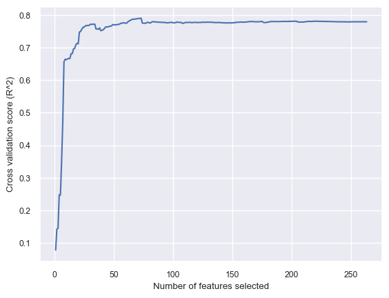
../_images/cf12f29d1f98868d30b4bd2a5e915c076446f0c27f9d0fafa6e2f87fff80bfe3.png

Our model is giving us the best results at number of features = 73.
But in our case when we pass these 73 selected features to RandomForestRegressor, which is a non-linear model, the scores get worse compared to 120 features or model-based selection. That said, we have reduced the dimensionality a lot.
This is similar to using cross-validation to tune a hyperparameter.
Indeed, the number of selected features is a hyperparameter.

`sklearn` `feature_importances_`#

Do we have to use Ridge for feature selection?
Many sklearn models have feature_importances_ attribute.
For tree-based models it’s calculated based on impurity (gini index or information gain).
For example, you can use RandomForestClassifier for feature selection. It will use feature_importances_ attribute instead of coefficients.

❓❓ Questions for you#

iClicker Exercise 4.1#

iClicker cloud join link: https://join.iclicker.com/C0P55

Select the below.

(A) Simple association-based feature selection approaches do not take into account the interaction between features.
(B) You can carry out feature selection using linear models by pruning the features which have very small weights (i.e., coefficients less than a threshold).
(C) Forward search is guaranteed to find the best feature set.
(D) RFE and backward selection are basically the same.
(E) The order of features removed given by rfe.ranking_ is the same as the order of original feature importances given by the model.

V’s answers: A, B

Summary#

What did we learn today?

Feature importances
Limitations of correlation based methods.
How to interpret coefficients of different types of features
Why do we need feature selection?
Model based feature selection
Recursive feature elimination
Forward/backward selection

We started with building a preliminary supervised machine learning pipeline in DSCI 571.
Now we are refining the pipeline by adding more components in it.

Coming up#

Model selection with complexity penalty
Regularization

(Optional) Problems with feature selection#

The term ‘relevance’ is not clearly defined.
What all things can go wrong with feature selection?
Attribution: From CPSC 340.

Example: Is “Relevance” clearly defined?#

Consider a supervised classification task of predicting whether someone has particular genetic variation (SNP)

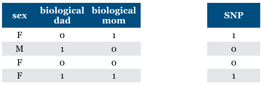
True model: You almost have the same value as your biological mom.

Is “Relevance” clearly defined?#

True model: You almost have the same value for SNP as your biological mom.
- (SNP = biological mom) with very high probability
- (SNP != biological mom) with very low probability

Is “Relevance” clearly defined?#

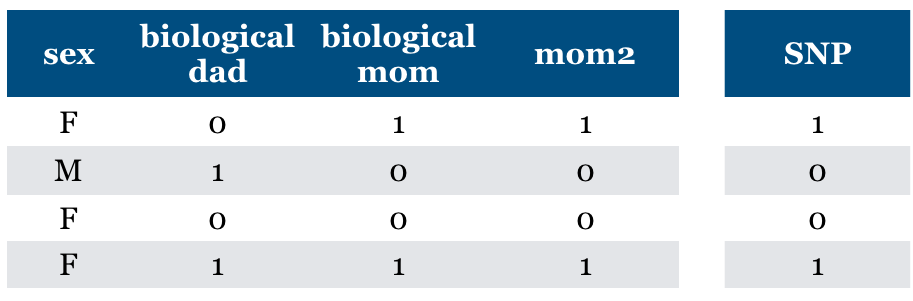
What if “mom” feature is repeated?
Should we pick both? Should we pick one of them because it predicts the other?
Dependence, collinearity for linear models
- If a feature can be predicted from the other, don’t know which one to pick.

Is “Relevance” clearly defined?#

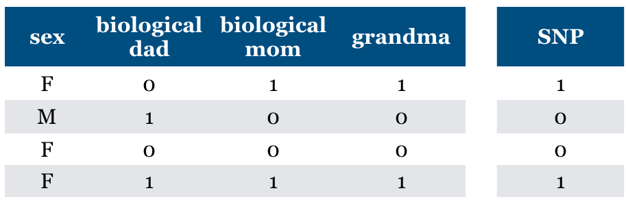
What if we add (maternal) “grandma” feature?
Is it relevant?
- We can predict SNP accurately using this feature
Conditional independence
- But grandma is irrelevant given biological mom feature
- Relevant features may become irrelevant given other features

Is “Relevance” clearly defined?#

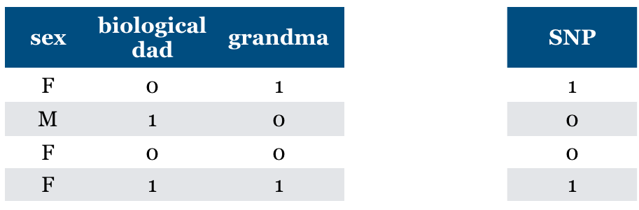
What if we do not know biological mom feature and we just have grandma feature
It becomes relevant now.
- Without mom feature this is the best we can do.
General problem (“taco Tuesday” problem)
- Features can become relevant due to missing information

Is “Relevance” clearly defined?#

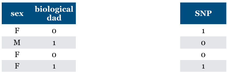
Are there any relevant features now?
They may have some common maternal ancestor.
What if mom likes dad because they share SNP?
General problem (Confounding)
- Hidden features can make irrelevant features relevant.

Is “Relevance” clearly defined?#

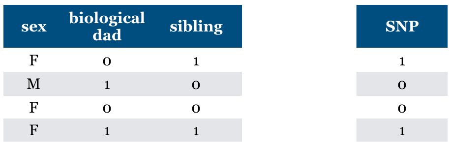
Now what if we have “sibling” feature?
The feature is relevant in predicting SNP but not the cause of SNP.
General problem (non causality)
- the relevant feature may not be causal

Is “Relevance” clearly defined?#

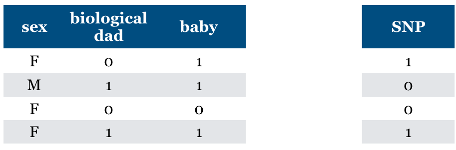
What if you are given “baby” feature?
Now the sex feature becomes relevant.
- “baby” feature is relevant when sex == F
General problem (context specific relevance)
- adding a feature can make an irrelevant feature relevant

Warnings about feature selection#

A feature is only relevant in the context of other features.
- Adding/removing features can make features relevant/irrelevant.
Confounding factors can make irrelevant features the most relevant.
If features can be predicted from other other features, you cannot know which one to pick.
Relevance for features does not have a causal relationship.
Is feature selection completely hopeless?
- It is messy but we still need to do it. So we try to do our best!

Lecture 4: Feature importances and feature selection

Contents

Lecture 4: Feature importances and feature selection#

Imports and LOs#

Imports#

Learning outcomes#

Data#

Let’s separate X and y#

Let’s identify feature types#

Feature importances#

SimpleFeature correlations#

Feature importances in linear models#

Ordinal features#

Categorical features#

Interpreting coefficients of numeric features#

Example showing how can we interpret coefficients of scaled features.#

Interim summary#

Feature selection: Introduction and motivation#

What is feature selection?#

Why feature selection?#

How do we carry out feature selection?#

Break (5 min)#

Feature selection using feature importances#

Model-based feature selection#

Recursive feature elimination (RFE)#

RFE algorithm#

Feature selection and categorical features#

(Optional) Feature selection and OHE#

RFE with cross-validation (RFECV)#

sklearn feature_importances_#

Search and score methods#

General idea of search and score methods#

Forward or backward selection#

Other ways to search#

Warnings about feature selection#

General advice on finding relevant features#

❓❓ Questions for you#

iClicker Exercise 4.1#

Summary#

Coming up#

(Optional) Problems with feature selection#

Example: Is “Relevance” clearly defined?#

Is “Relevance” clearly defined?#

Is “Relevance” clearly defined?#

Is “Relevance” clearly defined?#

Is “Relevance” clearly defined?#

Is “Relevance” clearly defined?#

Is “Relevance” clearly defined?#

Is “Relevance” clearly defined?#

Warnings about feature selection#

Relevant resources#

Let’s separate `X` and `y`#

`sklearn` `feature_importances_`#