

Lecture 5: Loss functions, intro to regularization#
UBC Master of Data Science program, 2022-23
Instructor: Varada Kolhatkar
Imports#
import os
import sys

sys.path.append("code/.")

%matplotlib inline
import matplotlib.pyplot as plt
import mglearn
import numpy as np
import numpy.random as npr
import pandas as pd

from plotting_functions import *
from sklearn import datasets
from sklearn.dummy import DummyClassifier, DummyRegressor
from sklearn.impute import SimpleImputer
from sklearn.linear_model import LinearRegression, LogisticRegression, Ridge, RidgeCV
from sklearn.model_selection import cross_val_score, cross_validate, train_test_split
from sklearn.preprocessing import PolynomialFeatures, StandardScaler

%matplotlib inline

pd.set_option("display.max_colwidth", 200)
Learning outcomes#
From this lecture, students are expected to be able to:
State the three important steps in supervised machine learning.
Broadly explain the concept of loss functions.
State the loss function of linear regression.
Broadly explain the effect of using ordinary least squares vs. absolute value loss function.
Explain why ordinary least squares is not a suitable loss function for classification problems.
Explain the trick of using \(y_iw^Tx_i\) when defining loss functions for classification problems.
Broadly explain the intuition behind 1/0, exponential, hinge and logistic loss.
Explain the difference between sigmoid and logistic loss.
Explain the general idea of complexity penalties.
Relate feature selection to the idea of complexity penalty.
Explain the general idea of L0 and L2 regularization.
Loss functions: big picture#
In DSCI 571, we primarily focused on how predict works. In this lecture, we’ll talk a bit about how fit works, primarily in the context of linear models.
In supervised machine learning we learn a mapping function which relates X to y. How do we learn this function?
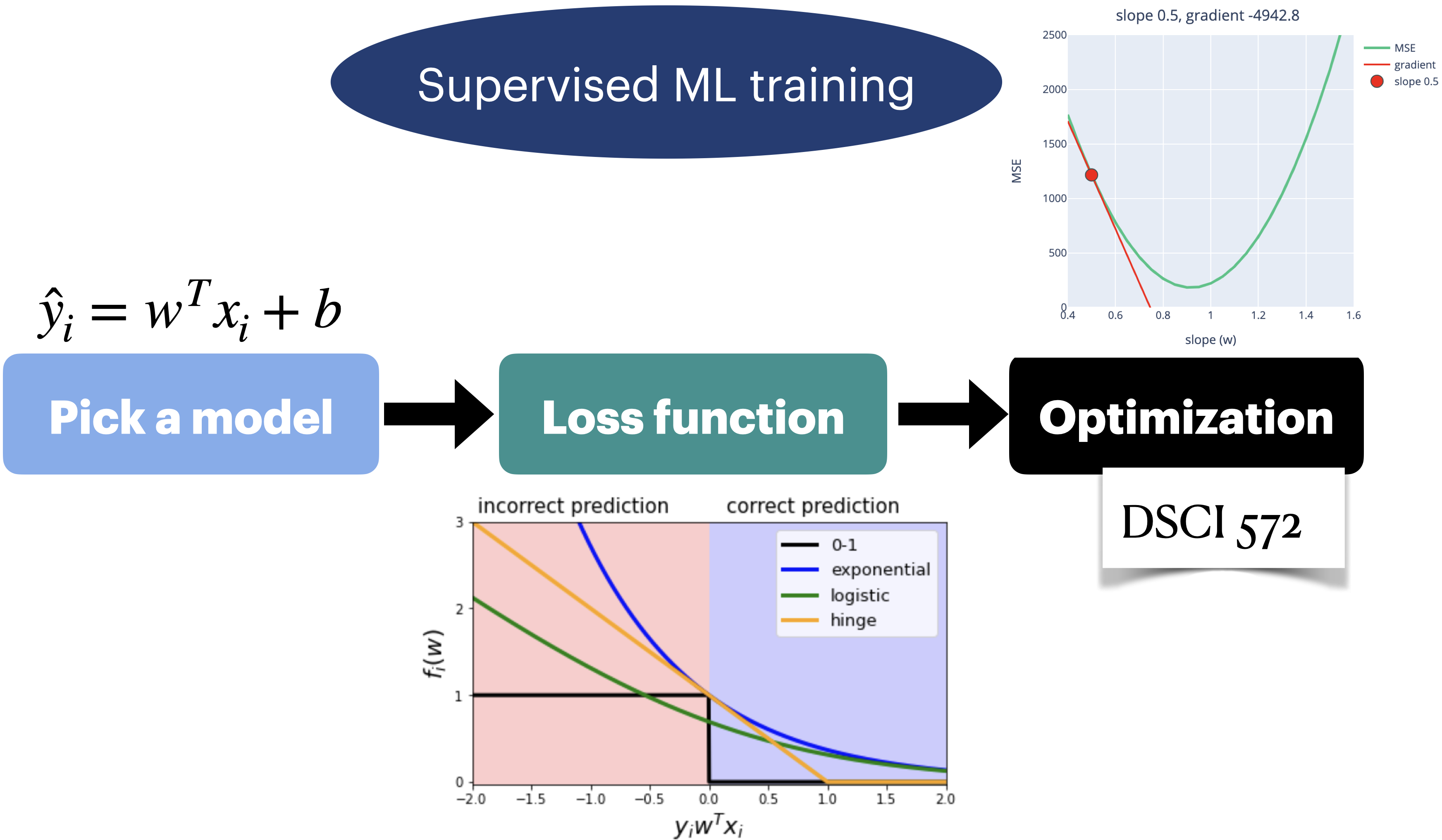
We can start to think of (a lot of) ML as a 3-step process:
Choose your model
Choose your loss function
Choose your optimization algorithm
Choosing your model#
What kind of mapping function do you want to learn?
Suppose we decide to go with a linear model. Then the possible mapping functions to choose from are only going to be linear functions.
Example: \(\hat{y}=5x_1+ 2x_2 - x_3\) or \(\hat{y}=10x_1+2x_2\)
Choosing your loss function#
We define a criteria to quantify how bad the model’s prediction is in comparison to the truth. This is called a loss function usually denoted as: \(\mathcal{l}(y, \hat{y})\).
Examples:
Binary classification: \(\mathcal{l}(y, \hat{y}) = \begin{cases} 0 \text{ if } y = \hat{y} \\ 1, \text{otherwise}\end{cases}\)
Regression: \(\mathcal{l}(y, \hat{y}) = (y-\hat{y})^2\)
Quantifies unhappiness of the fit across the training data.
Captures what is important to learn.
Using our loss function and our training data, we can examine which model function is better
Example: Which linear function is better for the given problem: \(\hat{y}=5x_1+ 2x_2 - x_3\) or \(\hat{y}=10x_1+2x_2\)?
Choosing your optimization algorithm#
Our goal is finding the optimal parameters so that the model’s predictions are least bad compared to the truth.
The optimization algorithm computationally finds the minimum of the loss function.
More on this in DSCI 572.
Linear regression loss function#
In the context of linear regression, when we call fit, a hyperplane is learned by the model. Let’s look at a toy example.
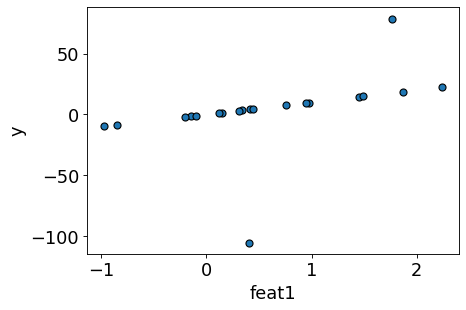
Consider this toy regression dataset with only one feature.
X_toy, y_toy = gen_outlier_data() # user-defined function in plotting_functions.py
plot_reg(X_toy, y_toy) # user-defined function in plotting_functions.py
Let’s train sklearn’s LinearRegression and get the regression line.
lr = LinearRegression()
lr.fit(X_toy, y_toy)
plot_reg(X_toy, y_toy, preds=lr.predict(X_toy), line=True)
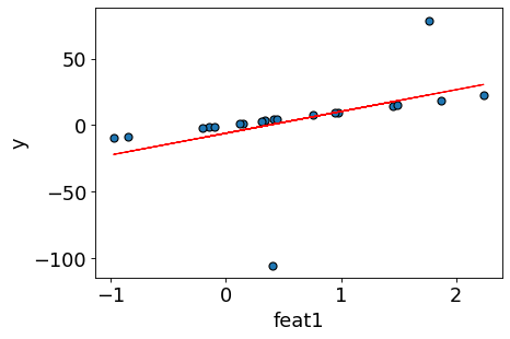
There could be many possible lines.
Why did linear regression pick this particular line?
Is this the “best” possible line?
Ordinary least squares#
Linear regression selected the above line by minimizing the quadratic cost between the actual target \(y\) and the model predictions \(\hat{y}\).
Where,
\(n \rightarrow\) number of examples
\(w \rightarrow\) weight vector (column vector)
This is called ordinary least squares (OLS), the most commonly used loss function or cost function for linear regression.
We define loss of a single example as squared difference between prediction and true target.
The total loss is summation of losses over all training examples.
Note: In this course all vectors are assumed to be column vectors.
Learning with OLS#
Among all possible lines, it will decide the “best” line by learning parameters \(w\) which make predictions for each training example as close as possible to the true \(y\) according to the loss function.
So once you decide what kind of model you are going to train, you can think of fit as a two-step process.
We need two things:
Loss function: A metric to measure how much a prediction differs from the true \(y\).
Optimization algorithm: for iteratively updating the weights so as to minimize the loss function. (You’ll talk about this in detail in 572.)
In 1D (only one feature in X), we will be learning two parameters: \(w_1\) and \(w_2\) (\(\beta_1, \beta_2\) in the picture below)
Our loss function will look like a bowl.
The contour plot projected on 2D looks like ellipses.
(Optional) For a well-defined ordinary least squares, there is a unique solution and it can be calculated analytically. $\(w_{OLS}= (X^TX)^{-1}X^Ty\)$
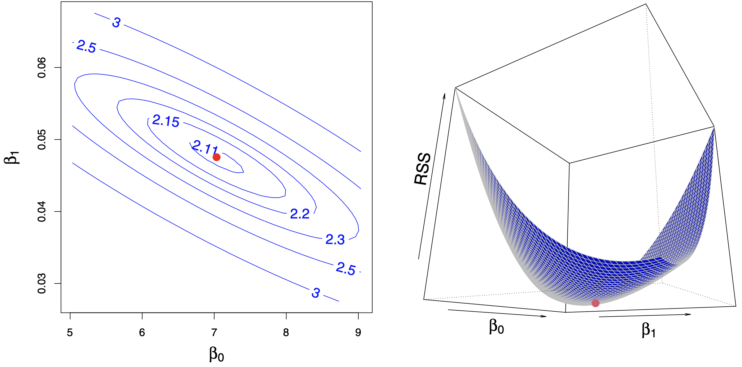 Source: https://www.statlearning.com/
Let’s experiment with different loss functions.
def lr_loss_squared(w, X, y): # define OLS loss function
    return np.sum((y - X @ w) ** 2)
Let’s use an optimizer from scipy.optimize and get the learned parameters.
from scipy.optimize import minimize # scipy optimizer
X_1 = np.concatenate((np.ones(X_toy.shape), X_toy), axis=1) # Create a column of ones
w_min = minimize(lr_loss_squared, np.zeros(2), args=(X_1, y_toy)).x # minimize the loss function defined above using an optimizer
print("scipy.optimize weights: ", w_min[1])
print("scipy.optimize intercept: ", w_min[0])
scipy.optimize weights:  16.342238893263442
scipy.optimize intercept:  -6.017153240936053
# user-defined function in plotting_functions.py
compare_regression_lines(X_toy, y_toy, lr.predict(X_toy), X_1@w_min)
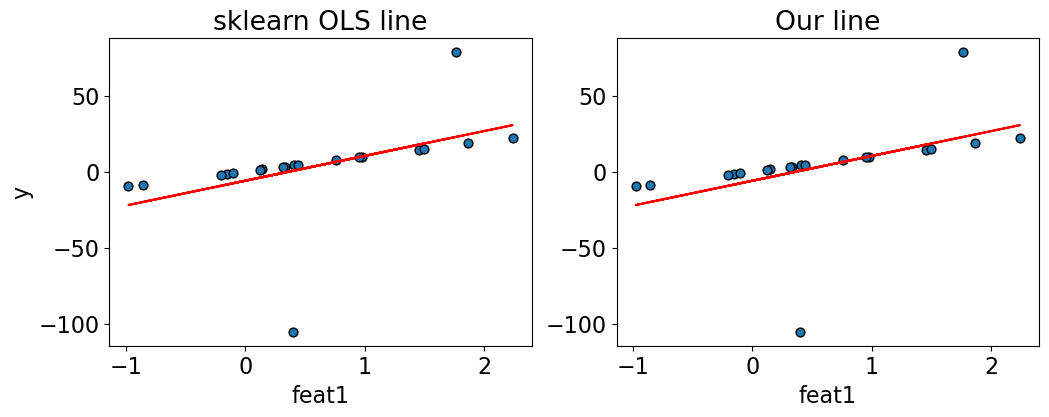
The sklearn OLS line and our OLS line are exactly the same!
Squared error loss penalizes really heavily for big errors compared to the absolute loss.
If you have a data point with a big error, the loss function is going to focus a lot on it as the penalty is very high for this this data point.
Absolute value loss#
An example of a different loss function would be the absolute value loss where we do not punish large errors as severely as ordinary least squares.
What are the implications of switching between these different choices?
Let’s try it out.
def lr_loss_abs(w, X, y):
    return np.sum(np.abs(y - X @ w))
w_min_abs = minimize(
    lr_loss_abs, np.zeros(2), args=(X_1, y_toy)
).x  # don't try this at home
compare_regression_lines(X_toy, y_toy, lr.predict(X_toy), X_1@w_min_abs)
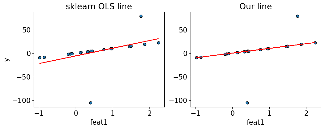
So, it seems like we got very different fits by changing the loss function.
In this case, the absolute loss gave us robust regression.
The loss function you pick is important!
Note: You will talk about robust regression in DSCI 561/562 and you’ll learn the maximum likelihood interpretation of the loss in DSCI 562.
Loss functions in classification problems#
How about using OLS for binary classification?#
Let’s assume binary classification with two classes: +1 and -1.
So \(y_i\) values are just +1 or -1.
The raw model output \(w^Tx_i\) can be any number.
Does it make sense to use this loss function for binary classification?
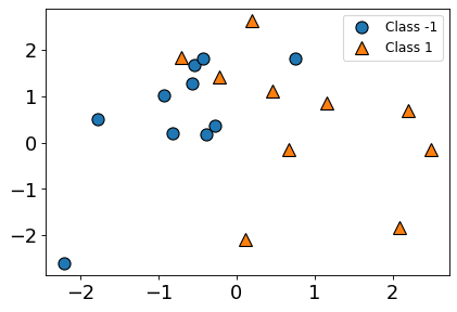
from sklearn.datasets import make_classification
X_classif, y_classif = make_classification(20, n_features=2, n_informative=2, n_redundant=0, random_state=122)
y_classif[y_classif == 0] = -1
plt.figure(figsize=(6, 4), dpi=80)
mglearn.discrete_scatter(X_classif[:, 0], X_classif[:, 1], y_classif)
plt.legend(["Class -1", "Class 1"], loc=1, fontsize=11);
logreg = LogisticRegression()
logreg.fit(X_classif, y_classif)
LogisticRegression()In a Jupyter environment, please rerun this cell to show the HTML representation or trust the notebook.
On GitHub, the HTML representation is unable to render, please try loading this page with nbviewer.org.
LogisticRegression()
plt.figure(figsize=(6, 4), dpi=80)
mglearn.discrete_scatter(X_classif[:, 0], X_classif[:, 1], y_classif)
plt.legend(["Class -1", "Class 1"], loc=1, fontsize=11)
mglearn.plots.plot_2d_separator(
    logreg, X_classif, eps=0.5, alpha=0.5
)
point1 = [2.48458573, -0.15474787]
point2 = [-0.22636803,  1.41418926]
plt.annotate("point1", point1, [point1[0] - 0.4,point1[1] + 0.2]);
plt.annotate("point2", point2, [point2[0] - 0.1, point2[1] + 0.1]);
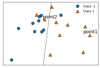
The model seems to be correct and confident about point1.
The model seems to be incorrect about point2
Should the loss for point1 be higher or lower than point2?
Let’s calculate least square losses for these points.
For point1, the correct prediction \(y_i\) is 1. So \((y_i - w^Tx_i)^2\) will be
(1 - logreg.coef_.ravel()@point1 + logreg.intercept_)**2
array([4.82807419])
For point2, the correct prediction \(y_i\) is again 1. So \((y_i - w^Tx_i)^2\) will be
(1 - logreg.coef_.ravel()@point2 + logreg.intercept_)**2
array([2.33661675])
Does it make sense?
Is this loss function capturing what we want it to capture?
What should be the loss? (Activity: 4 mins)#
Consider the following made-up classification example where target (true
y) is binary: -1 or 1.The true \(y\) (
y_true) and models raw scores (\(w^Tx_i\)) are given to you.You want to figure out how do you want to punish the mistakes made by the current model.
How will you punish the model in each case?
data = {
    "y_true": [1, 1, 1, 1, -1, -1, -1, -1],
    "raw score ($w^Tx_i$)": [10.0, 0.51, -0.1, -10, -12.0, -1.0, 0.4, 18.0],
    "correct? (yes/no)":["yes", "yes", "no", "no", "yes", "yes", "no", "no"],
    "confident/hesitant?":["confident", "hesitant", "hesitant", "confindent", "confident", "hesistant", "hesitant", "confident"],
    "punishment":["None", "small punishment", "", "", "", "", "", ""]
}
pd.DataFrame(data)
| y_true | raw score ($w^Tx_i$) | correct? (yes/no) | confident/hesitant? | punishment | |
|---|---|---|---|---|---|
| 0 | 1 | 10.00 | yes | confident | None |
| 1 | 1 | 0.51 | yes | hesitant | small punishment |
| 2 | 1 | -0.10 | no | hesitant | |
| 3 | 1 | -10.00 | no | confindent | |
| 4 | -1 | -12.00 | yes | confident | |
| 5 | -1 | -1.00 | yes | hesistant | |
| 6 | -1 | 0.40 | no | hesitant | |
| 7 | -1 | 18.00 | no | confident |
What do we want?#
Need a loss that encourages
\(w^Tx_i\) to be positive when \(y_i\) is \(+1\)
\(w^Tx_i\) to be negative when \(y_i\) is \(-1\)
Key idea#
Consider the product \(y_iw^Tx_i\).
We always want this quantity to be positive because
If \(y_i\) and \(w^Tx_i\) have the same sign, the product will be positive.
\(w^Tx_i\) is positive and \(y_i\) is positive 🙂
\(w^Tx_i\) is negative and \(y_i\) is negative 🙂
If they have oppositve signs, the product will be negative.
\(w^Tx_i\) is positive and \(y_i\) is negative 😔
\(w^Tx_i\) is negative and \(y_i\) is positive 😔
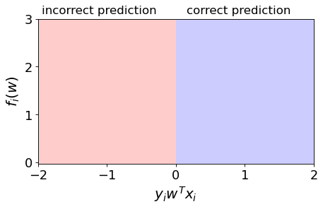
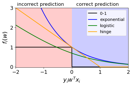
We’ll see this type of plots, where we plot \(y_iw^Tx_i\) vs. the loss \(f_i(w)\) for point \(x_i\).
Shows loss for one example.
plot_loss_diagram();
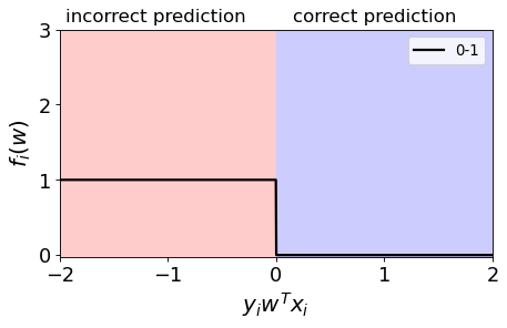
0/1 loss#
Binary state of happiness.
We are happy (loss=0) when the \(y_iw^Tx_i \geq 0\) $\(y_iw^Tx_i \geq 0, f_i(w) = 0\)$
We are unhappy (loss=1) when \(y_iw^Tx_i < 0\) $\(y_iw^Tx_i < 0, f_i(w) = 1\)$
grid = np.linspace(-2, 2, 1000)
plot_loss_diagram()
plt.plot(grid, grid < 0, color="black", linewidth=2, label="0-1")
plt.legend(loc="best", fontsize=12);
Preferences#
In 0/1 loss we are giving the same penalty to the examples where we are only slightly incorrect vs very incorrect.
It might be nice to have some preferences:
correct and confident (positive value with big magnitude of \(y_iw^Tx_i\))
> correct and hesitant (positive value with small magnitude of \(y_iw^Tx_i\))
> incorrect and hesitant (negative value with small magnitude of \(y_iw^Tx_i\))
> incorrect and confident (negative value with big magnitude of \(y_iw^Tx_i\))
Exponential loss#
Punish the wrong predictions exponentially. $\(\exp(-y_iw^Tx_i)\)$
plot_loss_diagram()
plt.plot(grid, grid < 0, color="black", linewidth=2, label="0-1") # 0-1 loss
plt.plot(grid, np.exp(-grid), color="blue", linewidth=2, label="exponential") # exponential loss
plt.legend(loc="best", fontsize=12);
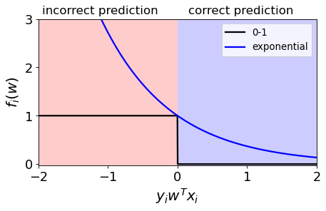
Intuition#
The function gets smaller as \(y_iw^Tx_i\) gets larger, so it encourages correct classification.
So if we minimize this loss, which means if we move down and to the right, it is encouraging positive values and hence correct predictions.
Hinge Loss#
Confident and correct examples are not penalized
Grows linearly for negative values in a linear fashion.
plot_loss_diagram()
plt.plot(grid, grid < 0, color="black", linewidth=2, label="0-1")
plt.plot(grid, np.exp(-grid), color="blue", linewidth=2, label="exponential")
plt.plot(grid, np.maximum(0, 1 - grid), color="orange", linewidth=2, label="hinge")
plt.legend(loc="best", fontsize=12);
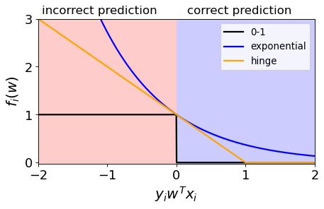
When you use Hinge loss with L2 regularization (coming up), it’s called a linear support vector machine.
$\(f(w) = \sum_{i=1}^n max\{0,1-y_iw^Tx_i\} + \frac{\lambda}{2} \lVert w\rVert_2^2\)$For more mathematical details on these topics see the following slide decks from CPSC 340.
It will make more sense when you learn about optimization in DSCI 572.
Logistic loss (logloss)#
Used in logistic regression
Grows linearly for negative values which makes it less sensitive to outliers.
\[\log\left(1+\exp(-y_iw^Tx_i)\right)\]
plot_loss_diagram()
plt.plot(grid, grid < 0, color="black", linewidth=2, label="0-1")
plt.plot(grid, np.exp(-grid), color="blue", linewidth=2, label="exponential")
plt.plot(grid, np.log(1 + np.exp(-grid)), color="green", linewidth=2, label="logistic")
plt.plot(grid, np.maximum(0, 1 - grid), color="orange", linewidth=2, label="hinge")
plt.legend(loc="best", fontsize=13);
Sigmoid vs. logistic loss#
A common source of confusion:
Sigmoid: \(\frac{1}{(1+\exp(-z))}\)
logistic loss: \(\log(1+\exp(-z))\)
They look very similar and both are used in logistic regression.
They have very different purposes.
sigmoid = lambda x: 1 / (1 + np.exp(-x))
raw_model_output = np.linspace(-8, 8, 1000)
plt.figure(figsize=(6, 4), dpi=80)
plt.plot(raw_model_output, sigmoid(raw_model_output))
plt.plot([0, 0], [0, 0.5], "--k")
plt.plot([-8, 0], [0.5, 0.5], "--k")
plt.xlabel("raw model output, $w^Tx$")
plt.ylabel("predicted probability")
plt.title("the sigmoid function");
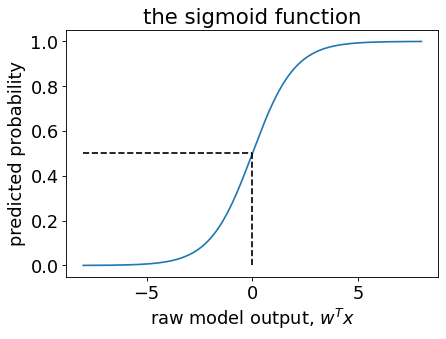
Sigmoid vs. logistic loss#
Sigmoid function: $\(\frac{1}{(1+\exp(-z))}\)$
Maps \(w^Tx_i\) to a number in \([0,1]\), to be interpreted as a probability.
This is important in
predict_proba.
Logistic loss: \(\log(1+\exp(-z))\)
Maps \(y_iw^Tx_i\) to a positive number, which is the loss contribution from one training example.
This is important in
fit.
(Optional) Another source of confusion#
Although this looks very different than the loss function we saw before, they produce the same loss.
This is also referred to as cross-entropy loss.
Logistic loss = cross-entropy loss
(Optional) The key difference between them#
This formulation assumes the classes to be 0 and 1. $\(f(w) = \sum_{x,y \in D} -y log(\hat{y}) - (1-y)log(1-\hat{y})\)$
Our previous formulation assumes classes to be -1 and +1. $\(f(w)=\sum_{i=1}^n\log\left(1+\exp(-y_iw^Tx_i)\right)\)$
Which loss function should I use?#
This part is more of an art than science.
What kind of penalty I want to put on the examples which are far away from the truth?
Many other loss functions available out there
ML researchers come up with their own loss functions based on their needs.
Break (~5 mins)#

Regularization: Motivation and notation#
Complex models and the fundamental tradeoff#
We’ve said that complex models tend to overfit more.
Recall: polynomial degree and train vs. validation scores.
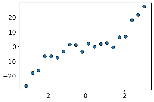
Let’s generate some synthetic data
n = 20
np.random.seed(4)
X_train = np.linspace(-3, 3, n)
y_train = X_train**3 + npr.randn(n) * 3

n = 20
X_valid = np.linspace(-3, 3, n)
y_valid = X_valid**3 + npr.randn(n) * 3

# transforming the data to include another axis
X_train = X_train[:, np.newaxis]
y_train = y_train[:, np.newaxis]

X_valid = X_valid[:, np.newaxis]
y_valid = y_valid[:, np.newaxis]

# plt.scatter(X_train, y_train, color="blue")
plt.figure(figsize=(6, 4))
mglearn.discrete_scatter(X_train, y_train, s=8);
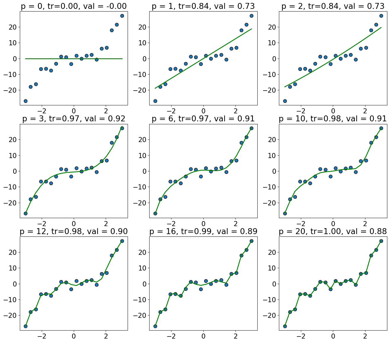
Let’s fit polynomials of different degrees on the synthetic data.
import panel as pn
from panel import widgets
from panel.interact import interact

pn.extension()

def f(degree=1):
    plot_poly_deg(X_train, y_train, X_valid, y_valid, degree=degree, valid=True)

interact(f, degree=widgets.IntSlider(start=1, end=20, step=1, value=1))
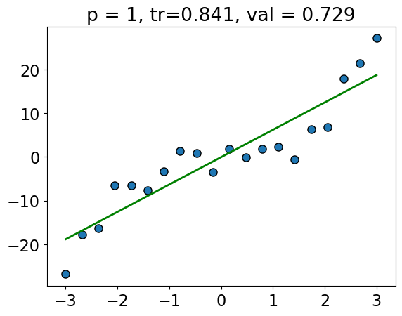
The training score goes up as we increase the degree of the polynomial, and is highest for \(p = 19\).
The validation score first goes up and then down.
The validation score is highest for \(p = 3\), and it goes down as we increase the degree after that; we start overfitting after \(p=3\).
plot_train_valid_poly_deg(X_train, y_train, X_valid, y_valid)
So there is a tradeoff between complexity of models and the validation score.
But what if we need complex models?
In supervised ML we try to find the mapping between \(X\) and \(y\), and usually the “true” mapping from \(X\) to \(y\) is complex.
Might need high-degree polynomial.
Might need to use many features, and don’t know “relevant” ones.
Controlling model complexity#
A few methods to control complexity:
Reduce the number of features (feature selection)
Model averaging (coming up): average over multiple models to decrease variance (e.g., random forests)

Regularization intuition#
Another popular method to control model complexity is by adding a penalty on the complexity of the model
Instead of minimizing just the Loss, we will minimize Loss + \(\lambda \) Model complexity
Loss term measures how well the model fits the data.
Model complexity term, which is also referred to as regularization term, measures model complexity.
A scalar \(\lambda\) decides the overall impact of the regularization term.
How to quantify model complexity?#
Total number of features with non-zero weights
L0 regularization: quantify model complexity as \(\lVert w \rVert\), L0 norm of \(w\).
As a function of weights: A feature weight with high absolute value is more complex than the feature weight with low absolute value.
L2 regularization: quantify model complexity as \(\lVert w \rVert_2^2\), square of the L2 norm of \(w\).
L1 regularization: quantify model complexity as \(\lVert w \rVert_1\), L1 norm of \(w\).
Terminology and notation#
Reminder: L0, L1, and L2 norms#
Given a vector \(w\),
L0 norm \(\lVert w \rVert \rightarrow\) the number of non-zero elements in \(w\)
L1 norm \(\lVert w \rVert_1 = \lvert w_1 \rvert + \lvert w_2 \rvert + \dots + \lvert w_n \rvert\)
L2 norm \(\lVert w \rVert_2 = (w_1^2 + w_2^2 + \dots + w_n^2)^{1/2}\)
Square of the L2 norm \(\lVert w \rVert_2^2 = (w_1^2 + w_2^2 + \dots + w_n^2)\)
from numpy import array
from numpy.linalg import norm

w = array([0, -2, 4])

l0 = norm(w, 0)  # number of non-zero values
l1 = norm(w, 1)  # sum of absolute values
l2 = norm(w, 2)  # square root of sum of the squared values
print("The l0 norm of %s is: %0.3f" % (w, l0))
print("The l1 norm of %s is: %0.3f" % (w, l1))
print("The l2 norm of %s is: %0.3f" % (w, l2))
The l0 norm of [ 0 -2  4] is: 2.000
The l1 norm of [ 0 -2  4] is: 6.000
The l2 norm of [ 0 -2  4] is: 4.472
# norms of a vector
from numpy import array
from numpy.linalg import norm

w = array([0, -2, 3, 0])
# l0 norm is the number of non-zero values in a vector
print("The l0 norm of %s is: %0.3f" % (w, norm(w, 0)))

# l1 norm is the sum of the absolute values in a vector.
print("The l1 norm of %s is: %0.3f" % (w, norm(w, 1)))

# l2 norm is square root of the sum of the squared values in a vector.
print("The l2 norm of %s is: %0.3f" % (w, norm(w, 2)))
The l0 norm of [ 0 -2  3  0] is: 2.000
The l1 norm of [ 0 -2  3  0] is: 5.000
The l2 norm of [ 0 -2  3  0] is: 3.606
We can write least squares using this notation.
It’s the square of the L2 norm of the difference between predicted y’s and true y’s.
(Optional) Vectorization#
We can organize all the training examples into a matrix \(Z\) with one row per training example.
Then compute the predictions for the whole dataset succinctly as \(Zw\) for the whole dataset:
We take each row of \(Z\) and dot-product it with \(w\). So the result is a vector of all our predictions.
Sometimes, we refer to the transformed data (e.g., after applying polynomial transformations) as \(Z\) (instead of \(X\)) and the weights associated with the transformed features as \(v\) (instead of \(w\)).
So the least square loss function after applying polynomial transformations can be written as:
Complexity penalties and L0 regularization#
Model selection: complexity penalty#
We want our model to fit the data well but we do not want an overly complex model.
How about penalizing complex models?
compare_poly_degrees(3, 4, X_train, y_train, X_valid, y_valid) # user-defined function in plotting_functions.py
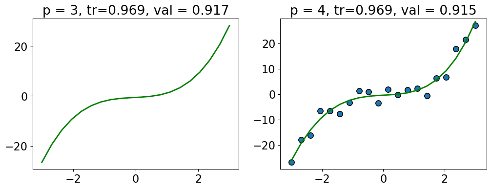
For example, here we are getting more or less the same scores with \(p=3\) and \(p=4\).
How about penalizing complex models a bit so that in such situation we would pick a simpler model?
Complexity penalty#
Measure complexity in terms of the number of degrees of freedom or parameters in the model
In case polynomial features, minimize the training error + the degree of polynomial.
Find \(p\) that minimizes
where
\(p \rightarrow\) degree of polynomial in polynomial transformations
\(Z_p \rightarrow\) transformed polynomial features
\(v \rightarrow\) weights associated with \(Z_p\)
If we use \(p=3\), use loss + 3 as the total loss.
If we use \(p=4\), use loss + 4 as the total loss.
If two \(p\) have similar losses, this prefers smaller \(p\).
Optimizing this score#
Form \(Z_0\), solve for \(v\) compute \( score(0) = \lVert{Z_0v -y}_2\rVert^2 + 0\)
Form \(Z_1\), solve for \(v\) compute \( score(1) = \lVert{Z_1v -y}\rVert^2 + 1\)
Form \(Z_2\), solve for \(v\) compute \( score(2) = \lVert{Z_2v -y}\rVert^2 + 2\)
Form \(Z_3\), solve for \(v\) compute \( score(3) = \lVert{Z_3v -y}\rVert^2 + 3\)
Choose the degree with the lowest score.
We need to decrease the training error by at least 1 to increase degree by 1.
(Optional) Model selection#
There are many scores usually with the form: $\( score(p) = \frac{1}{2}\lVert{Z_pv -y}\rVert^2 + \lambda k\)$
\(k\rightarrow \text{estimated parameters/degrees of freedom}\)
\(\lambda \rightarrow \text{penalization factor}\)
Pick the model with lowest score.
The way we choose \(\lambda\) gives us different statistical measures for model selection.
For example
AIC sets \(\lambda = 1\) and penalizes the model complexity by the degree of freedom
BIC sets \(\lambda = log(N)\), where \(N\) is the number of examples.
MSE does not penalize the model
Classification error does not penalize the model
More on these measures here. You’ll learn more about this in DSCI 562.
Remember the search and score methods for feature selection#
Define a scoring function \(f(S)\) that measures the quality of the set of features \(S\).
Now search for the set of features \(S\) with the best score.
Example: Suppose you have three features: \(A, B, C\)
Compute score for \(S = \{\}\)
Compute score for \(S = \{A\}\)
Compute score for \(S= \{B\}\)
Compute score for \(S = \{C\}\)
Compute score for \(S = \{A,B\}\)
Compute score for \(S = \{A,C\}\)
Compute score for \(S = \{B,C\}\)
Compute score for \(S = \{A,B,C\}\)
Return \(S\) with the best score.
Scoring using complexity penalties#
Find \(S\) and \(W_s\) minimizing the squared error + the number of selected features
\(X_{S}\) is features \(S\) of examples \(X\).
Example
Suppose \(S_1 = \{f_1, f_2, f_4\}\) \(S_2 = \{f_1, f_2, f_4, f_5\}\) have similar error, it prefers \(S_1\).
It prefers removing \(f_5\) instead of keeping it with a small weight.
Instead of \(size(S)\), we usually write “\(L0\) norm”.
\(L0\) “norm” and the number of features used#
In linear models, setting \(w_j = 0\) is the same as removing the feature.
Example: $\(\hat{y_i} = w_1x_1 + w_2x_2 + w_3x_3 + w_4x_4\)$
\(L0\) “norm” is the number of non-zero values.
If \(w = \begin{bmatrix}0.8 \\ 0.0 \\ 0.03 \\0.1\end{bmatrix}\), \(\lVert w\rVert_0 = 3\) and if \(w = \begin{bmatrix}0.0 \\ 0.0 \\ 0.22 \\0.0\end{bmatrix}\), \(\lVert w\rVert_0 = 1\)
Example#
Imagine the following two weight vectors which give the same error.
Which one would be chosen by L0 regularization?
\(\lVert w^1\rVert_0 = 1\) and \(\lVert w^2\rVert_0 = 2\). So it will pick \(w^1\).
Scoring using \(L0\) “norm”#
Most common “scores” have the form.
\(\lVert{Xw -y}\rVert^2_2 \rightarrow\) square of the L2 norm \(Xw -y\)
\(\lambda \rightarrow\) penalty parameter
\(\lVert w\rVert_0 \rightarrow\) L0 norm of \(w\)
The number of non-zero values in \(w\).
To increase the degrees of freedom by one, need to decrease the error by \(\lambda\).
Prefer smaller degrees of freedom if errors are similar.
Can’t optimize because the function is discontinuous in \(\lVert w\rVert_0\)
Search over possible models
L2 regularization#
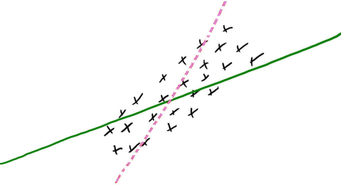
Idea of regularization: Pick the line/hyperplane with smaller slope#
Assuming red and green models have the same training error and if you are forced to choose one of them, which one would you pick?
Pick the solid green line because its slope is smaller.
Small change in \(x_i\) has a smaller change in prediction \(y_i\)
Since \(w\) is less sensitive to the training data, it’s likely to generalize better.
Standard regularization strategy is L2 regularization
We incorporate L2 penalty in the loss function \(f(w)\): $\(f(w) = \sum_i^n(w^Tx_i - y_i)^2 + \lambda\sum_j^d w_j^2 \text{ or }\)\( \)\(f(w) = \lVert Xw - y\rVert_2^2 + \lambda \lVert w\rVert_2^2\)$
\(\lVert Xw - y\rVert_2^2 \rightarrow\) square of the \(L2\) norm of \(Xw -y\)
\(\lambda \rightarrow\) regularization strength
\(\lVert w\rVert_2^2 \rightarrow\) square of the L2 norm of \(w\)
sum of the squared weight values.
L2 regularization#
Objective balances getting low error vs. having small slopes \(w_j\)
In terms of fundamental trade-off:
You can increase the training error.
Nearly-always reduces overfitting and the validation error.
Regularization demo#
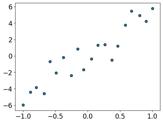
Let’s generate some synthetic data with N = 20 points.
np.random.seed(4)
N = 20
X = np.linspace(-1, 1, N) + npr.randn(N) * 0.01
X = X[:, None]
y = npr.randn(N, 1) + X * 5

mglearn.discrete_scatter(X, y, s=6, labels=["training data"]);
Let’s fit with degree \(N-1\) polynomial
pf = PolynomialFeatures(19)
Z = pf.fit_transform(X)

lr = LinearRegression()
lr.fit(Z, y)
w_lr_19 = lr.coef_.flatten()
grid = np.linspace(min(X), max(X), 1000)
grid_poly_19 = pf.fit_transform(grid)
plt.figure(figsize=(6,4))
mglearn.discrete_scatter(X, y, s=6, labels=["training data"])
plt.plot(grid, grid_poly_19 @ w_lr_19, c="red", linewidth=1);
lr.score(Z, y)
1.0
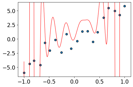
Problem: this results are crazy (overfitting).
Bigger values of weights means the model is very sensitive to the training data.
pd.DataFrame(w_lr_19, index=pf.get_feature_names_out(), columns=["weights"]).tail()
| weights | |
|---|---|
| x0^15 | -5.150150e+07 |
| x0^16 | -5.316861e+06 |
| x0^17 | 3.466582e+07 |
| x0^18 | 1.482311e+06 |
| x0^19 | -9.517721e+06 |
print(max(abs(w_lr_19)))
51501499.24478904
Solution 1: Use a lower degree polynomial#
pf = PolynomialFeatures(2)
Z = pf.fit_transform(X)
lr = LinearRegression()
lr.fit(Z, y)
w_lr_2 = lr.coef_.flatten()
grid_poly_2 = pf.fit_transform(grid)
plt.figure(figsize=(6,4))
mglearn.discrete_scatter(X, y, s=6, labels=["training data"])
plt.plot(grid, grid_poly_2 @ w_lr_2, c="red");
lr.score(Z, y)
0.8717193637247818
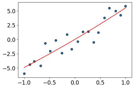
The lower degree polynomial looks good.
But if the true relationship really was complicated? Then if we restricted the degree of the polynomial, we’d miss out on it.
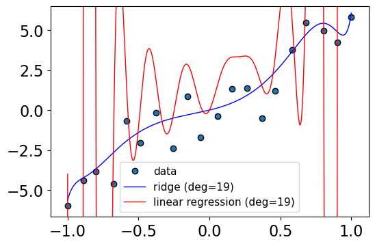
Solution 2: Use regularization#
The idea of regularization is to “regularize” weights so that they are small and so less sensitive to the data.
pf = PolynomialFeatures(19)
Z = pf.fit_transform(X)

r = Ridge(alpha=0.01)  # Regularized linear regression
r.fit(Z, y)
w_ridge_19 = r.coef_.flatten()
plt.figure(figsize=(6,4))
mglearn.discrete_scatter(X, y, s=6, labels=["training data"])
grid_poly_ridge = pf.fit_transform(grid)
plt.plot(grid, grid_poly_ridge @ w_ridge_19, c="blue", linewidth=1);
plt.plot(grid, grid_poly_19 @ w_lr_19, c="red", linewidth=1);
plt.legend(["data", 'ridge (deg=19)', 'linear regression (deg=19)'], loc="best", fontsize=11);
r.score(Z, y)
0.9135817441429818
pd.DataFrame(w_ridge_19, index=pf.get_feature_names_out(), columns=["weights"]).tail()
| weights | |
|---|---|
| x0^15 | 0.780600 |
| x0^16 | 1.170325 |
| x0^17 | 2.655623 |
| x0^18 | 1.800171 |
| x0^19 | 4.240822 |
print(max(abs(w_ridge_19)))
8.010363113222288
Regularization helped! Even though we used a degree \(N-1\) polynomial, we didn’t end up with a crazy model.
We are keeping all the complex features but assigning small weights to higher degree polynomial.
We can add regularization to many models, not just least squares with a polynomial basis.
Why are small weights better?#
Somewhat non-intuitive.
Suppose \(x_1\) and \(x_2\) are nearby each other.
We might expect that they have similar \(\hat{y}\).
If we change feature1 value by a small amount \(\epsilon\) in \(x_2\), leaving everything else the same, we might think that the prediction would be the same.
But if we have bigger weights small change in \(x_2\) has a large effect on the prediction.
x_1 = np.array([1, 1, 0, 1, 1, 0])
x_2 = np.array([0.8, 1, 0, 1, 1, 0])
weights = np.array([100, 0.1, 1, 0.22, 4, 3])

print("x_1 prediction: ", x_1.dot(weights))
print("x_2 prediction: ", x_2.dot(weights))
x_1 prediction:  104.32
x_2 prediction:  84.32
In linear models, the rate of change of the prediction function is proportional to the individual weights.
So if we want the function to change slowly, we want to ensure that the weights stay small.
The idea is to avoid putting all our energy into one features, which might give us over-confident predictions and lead to overfitting.
Have we seen L2 regularization before?#
Ridge: Linear Regression with L2 regularization
class sklearn.linear_model.Ridge(alpha=1.0, fit_intercept=True, normalize=False, copy_X=True, max_iter=None, tol=0.001, solver=’auto’, random_state=None)
Linear least squares with l2 regularization. Minimizes the objective function: ||y - Xw||^2_2 + alpha * ||w||^2_2 This model solves a regression model where the loss function is the linear least squares function and regularization is given by the l2-norm. Also known as Ridge Regression or Tikhonov regularization.
Uses the hyperparameter \(\alpha\) for regularization strength instead of \(\lambda\); larger value of \(\alpha\) means more regularization. $\(f(w) = \lVert Xw - y\rVert_2^2 + \alpha \lVert w\rVert_2^2\)$
LogisticRegression: Logistic Regression with L2 regularization
class sklearn.linear_model.LogisticRegression(penalty=’l2’, *, dual=False, tol=0.0001, C=1.0, fit_intercept=True, intercept_scaling=1, class_weight=None, random_state=None, solver=’lbfgs’, max_iter=100, multi_class=’auto’, verbose=0, warm_start=False, n_jobs=None, l1_ratio=None)
C: default=1.0 Inverse of regularization strength; must be a positive float. Like in support vector machines, smaller values specify stronger regularization.
Summary: What did we learn today?#
Loss functions (high level)
OLS vs absolute loss
0/1 loss
Exponential loss
Hinge loss
Logistic loss
Adding complexity penalties to the loss function
L0 penalty
Introduction to L2 regularization
Coming up
More on L2 regularization
L1 regularization
❓❓ Questions for you#
Exercise 5.1 L0 and L2-regularization#
Select all the statements below which are True.
(A) In the equation below of L0-regularization, smaller value for \(\lVert w\rVert_0\) means we discard most of the features. $\( f(w) = \lVert{Xw -y}\rVert^2 + \lambda \lVert w\rVert_0\)$
(B) In the above equation, larger \(\lambda\) means aggressively changing many weights to zero.
V’s answers: A, B,
Exercise 5.2#
Imagine that you fit Ridge twice with different values of \(\alpha\), \(\alpha = 0\) and \(\alpha=10\). You are given the weights learned from two different models below. Without knowing which weights came from which model, you can guess that \(w^1\) probably corresponds to \(\alpha = 10\) and \(w^2\) probably corresponds to \(\alpha = 0\).
V’s answers: False. Bigger alpha means the weights should be smaller.