Lecture 6: L2- and L1-Regularization

Lecture 6: L2- and L1-Regularization#

UBC Master of Data Science program, 2022-23

Instructor: Varada Kolhatkar

Atrribution: A lot of this material is adapted from CPSC 340 lecture notes.

Imports#

import os
import sys

sys.path.append("code/.")
%matplotlib inline
import matplotlib.pyplot as plt
import mglearn
import numpy as np
import numpy.linalg as npla
import numpy.random as npr
import pandas as pd
from plotting_functions import *
from sklearn import datasets
from sklearn.dummy import DummyClassifier, DummyRegressor
from sklearn.impute import SimpleImputer
from sklearn.linear_model import LinearRegression, LogisticRegression, Ridge, RidgeCV
from sklearn.model_selection import cross_val_score, cross_validate, train_test_split
from sklearn.preprocessing import PolynomialFeatures, StandardScaler
pd.set_option("display.max_colwidth", 200)

Learning outcomes#

From this lecture, students are expected to be able to:

Broadly explain L2 regularization (Ridge).
Use L2 regularization (Ridge) using sklearn.
Compare L0- and L2-regularization.
Explain the relation between the size of regression weights, overfitting, and complexity hyperparameters.
Explain the effect of training data size and effect of regularization.
Explain the general idea of L1-regularization.
Learn to be skeptical about interpretation of the coefficients.
Use L1-regularization (Lasso) using sklearn.
Discuss sparsity in L1-regularization.
Compare L0-, L1-, and L2-regularization.
Use L1 regularization for feature selection.
Explain the importance of scaling when using L1- and L2-regularization
Broadly explain how L1 and L2 regularization behave in the presence of collinear features.

Recap#

Idea of regularization: Pick the line/hyperplane with smaller slope#

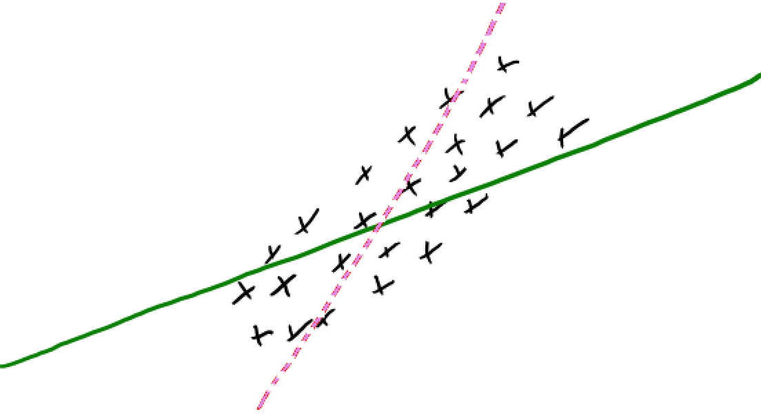
Assuming the models below (dashed and solid green lines) have the same training error and if you are forced to choose one of them, which one would you pick?
- Pick the solid green line because its slope is smaller.
- Small change in $x_i$ has a smaller change in prediction $y_i$
- Since $w$ is less sensitive to the training data, it’s likely to generalize better.

Regularization is a technique for controlling model complexity.
- Instead of minimizing just the Loss, minimize Loss + $\lambda $ Model complexity
- Loss: measures how well the model fits the data.
- Model complexity: measures model complexity (also referred to as regularization term)
- A scalar $\lambda$ decides the overall impact of the regularization term.

How to quantify model complexity?#

Total number of features with non-zero weights
- L0 regularization: quantify model complexity as $\lVert w \rVert_0$, L0 norm of $w$.
As a function of weights: A feature weight with high absolute value is more complex than the feature weight with low absolute value.
- L2 regularization: quantify model complexity as $\lVert w \rVert_2^2$, square of the L2 norm of $w$.
- L1 regularization: quantify model complexity as $\lVert w \rVert_1$, L1 norm of $w$.

L0-regularization#

L0-regularization.

\[f(w) = \lVert Xw - y\rVert_2^2 + \lambda \lVert w\rVert_0\]

Regularization parameter $\lambda$ controls the strength of regularization.
To increase the degrees of freedom by one, need to decrease the error by $\lambda$.
Prefer smaller degrees of freedom if errors are similar.
Can’t optimize because the function is discontinuous in $\lVert w\rVert_0$
- Search over possible models

L2-regularization#

Standard regularization strategy is L2-regularization.
Also referred to as Ridge.
The loss function has an L2 penalty term.

\[f(w) = \lVert Xw - y\rVert_2^2 + \lambda \lVert w\rVert_2^2\]

Regularization parameter $\lambda$ controls the strength of regularization.
- bigger $\lambda$ $\rightarrow$ more regularization $\rightarrow$ lower weights
Setting $\lambda = 0$ is the same as using OLS
- Low training error, high variance, bigger weights, likely to overfit
Setting $\lambda$ to a large value leads to smaller weights
- Higher training error, low variance, high bias, smaller weights, likely to underfit
We want to strike a balance between these two extremes, which we can control by optimizing the value for $\lambda$.

`sklearn`’s `Ridge` or L2 regularization#

Let’s bring back sklearn's California housing dataset.

from sklearn.datasets import fetch_california_housing
from sklearn.preprocessing import PolynomialFeatures

housing = fetch_california_housing(as_frame=True)
X = housing["data"]
y = housing["target"]

pf = PolynomialFeatures(degree=2, include_bias=False)
X = pf.fit_transform(X)
X_train_poly, X_test_poly, y_train, y_test = train_test_split(X, y, random_state=0)

ss = StandardScaler()
X_train = ss.fit_transform(X_train_poly)
X_test = ss.transform(X_test_poly)

X_train.shape

(15480, 44)

Let’s explore L2 regularization with this dataset.

Example: L2-Regularization “Shrinking”#

$\lambda$ in the formulation above is alpha in sklearn.
We get least squares with $\lambda = 0$.
As we increase $\alpha$
- $\lVert Xw - y\rVert_2^2$ goes $\uparrow$
- $\lVert w\rVert_2^2$ goes $\downarrow$
- Though individual $w_j$ can increase or decrease with lambda because we use the L2-norm, the large ones decrease the most.

def lr_loss_squared(w, X, y): # define OLS loss function
    return np.sum((y - X @ w) ** 2)

from numpy.linalg import norm
alphas = [0, 0.01, 0.1, 1.0, 10, 100, 1000, 1000000]
weight_shrinkage_data = {'alpha':[], '||Xw - y||^2':[], '||w||^2':[], 'intercept':[], 'train score':[], 'test score':[]}

for (i, alpha) in enumerate(alphas): 
    r = Ridge(alpha=alpha) 
    r.fit(X_train, y_train)
    weight_shrinkage_data['alpha'].append(alpha)
    OLS = np.round(lr_loss_squared(r.coef_, X_train, y_train), 4)
    l2_term = np.round(norm(r.coef_, 2)**2, 4)
    intercept = np.round(r.intercept_,4)
    weight_shrinkage_data['||Xw - y||^2'].append(OLS)
    weight_shrinkage_data['||w||^2'].append(l2_term)    
    weight_shrinkage_data['intercept'].append(intercept)
    weight_shrinkage_data['train score'].append(np.round(r.score(X_train, y_train), 2))
    weight_shrinkage_data['test score'].append(np.round(r.score(X_test, y_test), 2))

pd.DataFrame(weight_shrinkage_data)

	alpha	\|\|Xw - y\|\|^2	\|\|w\|\|^2	intercept	train score	test score
0	0.00	73099.4882	7634.4579	2.0744	0.69	-0.73
1	0.01	73113.1963	4239.9359	2.0744	0.69	-0.17
2	0.10	73222.8589	888.3987	2.0744	0.68	0.62
3	1.00	73437.3112	77.0152	2.0744	0.67	0.02
4	10.00	73597.9629	8.4983	2.0744	0.66	-3.80
5	100.00	73777.7373	2.5195	2.0744	0.65	-3.37
6	1000.00	74363.2804	0.7118	2.0744	0.62	0.10
7	1000000.00	85565.9420	0.0008	2.0744	0.08	0.08

In this example, as alpha goes up

$\lVert Xw - y\rVert_2^2$ is increasing
$\lVert w\rVert_2^2$ is decreasing; weight become smaller and smaller
The intercept stays the same. It’s the mean of the target – dummy model prediction.
We are getting best test score for alpha=0.10.
The total loss is worse than OLS but it’s helping with generalization.

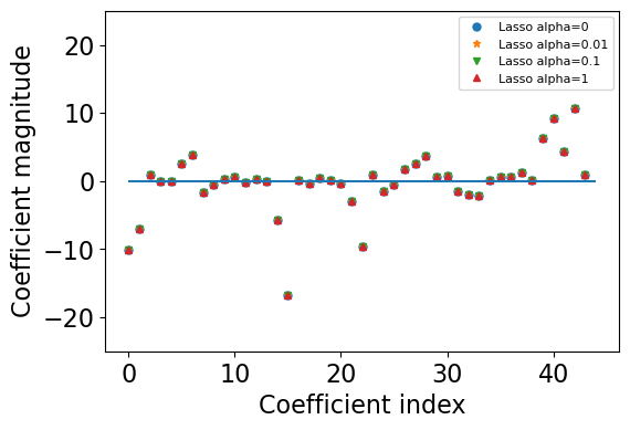
The weights become smaller but do not become zero#

As alpha goes up, we increase the regularization strength.
The weights become smaller and smaller but tend not to become exactly zero.

alphas = [0, 0.01, 1, 1000]

plt.figure(figsize=(6, 4))
markers = ['o','*', 'v','^']
ridge_models = {}
for (i, alpha) in enumerate(alphas):
    r = Ridge(alpha = alpha)
    r.fit(X_train, y_train)
    plt.plot(r.coef_, markers[i], markersize=5, label="Ridge alpha="+ str(alpha))
plt.xlabel("Coefficient index")
plt.ylabel("Coefficient magnitude")
plt.hlines(0, 0, len(r.coef_))
plt.ylim(-25, 25)
plt.legend(loc="best",fontsize=8);    

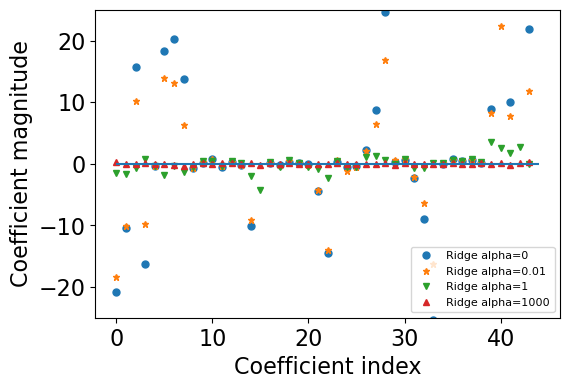
../_images/753649090a65ad77aa5f60605741348daee452ad75d372a6d2e7fe0added299a.png

Let’s try a very large alpha value, which is likely to make weights very small.

ridge10000 = Ridge(alpha=10000).fit(X_train, y_train)
print("Total number of features", X_train.shape[1])
print("Number of non-zero weights: ", np.sum(ridge10000.coef_ != 0))

Total number of features 44
Number of non-zero weights:  44

All features have non-zero weights.

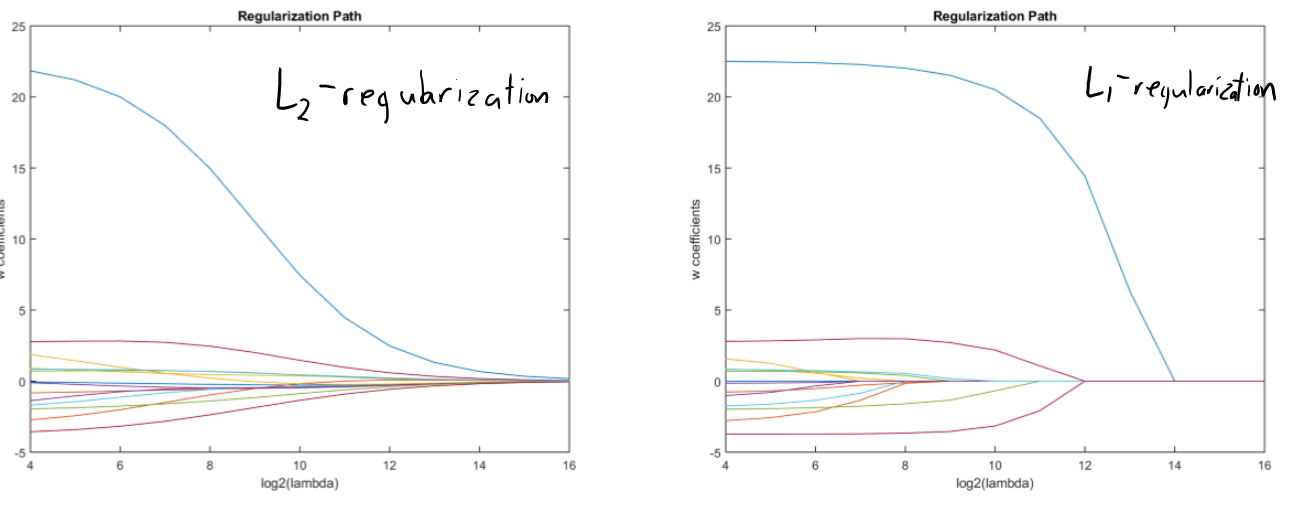
Regularization path#

Let’s trace the journey of coefficients of a few features with different values of alpha.

feature_names = pf.get_feature_names_out()

Let’s examine the coefficients

r10 = Ridge(alpha=0.10)
r10.fit(X_train, y_train)
coefs = (
    pd.DataFrame(r10.coef_, feature_names, columns=["coef"])
    .query("coef != 0")
    .sort_values("coef")
    .reset_index()
    .rename(columns={"index": "variable"})
)

coefs.style.background_gradient('PuOr')

	variable	coef
0	MedInc Longitude	-16.762873
1	MedInc	-10.178537
2	HouseAge Longitude	-9.608717
3	HouseAge	-6.986869
4	MedInc Latitude	-5.683734
5	HouseAge Latitude	-2.931366
6	AveBedrms Longitude	-2.152434
7	AveBedrms Latitude	-1.934514
8	Longitude	-1.637599
9	AveRooms AveBedrms	-1.571689
10	AveBedrms AveOccup	-1.536152
11	MedInc^2	-0.540772
12	AveRooms Population	-0.518624
13	HouseAge AveOccup	-0.414707
14	HouseAge AveRooms	-0.376728
15	MedInc AveBedrms	-0.280714
16	Population	-0.106295
17	MedInc AveOccup	-0.072894
18	AveBedrms	-0.067099
19	Population^2	0.050877
20	HouseAge Population	0.076735
21	AveOccup^2	0.177787
22	HouseAge^2	0.197444
23	MedInc HouseAge	0.292222
24	MedInc Population	0.358598
25	HouseAge AveBedrms	0.495107
26	MedInc AveRooms	0.544633
27	Population Latitude	0.573911
28	Population AveOccup	0.603423
29	AveBedrms^2	0.620403
30	AveBedrms Population	0.780217
31	AveRooms	0.908226
32	AveRooms^2	0.940577
33	Longitude^2	0.944154
34	Population Longitude	1.199605
35	AveRooms AveOccup	1.697423
36	AveOccup	2.478821
37	AveRooms Latitude	2.523284
38	AveRooms Longitude	3.693662
39	Latitude	3.830685
40	Latitude^2	4.330258
41	AveOccup Latitude	6.270548
42	AveOccup Longitude	9.143782
43	Latitude Longitude	10.627639

feats = ['MedInc', 'AveBedrms',  'Population', 'MedInc Longitude', 'Population Longitude', 'Latitude Longitude']

msk = [feat in feats for feat in feature_names]

#feature_names

r10.coef_[msk]

array([-10.17853657,  -0.06709887,  -0.10629543, -16.7628735 ,
         1.19960525,  10.6276393 ])

# Attribution: Code adapted from here: https://scikit-learn.org/stable/auto_examples/linear_model/plot_ridge_path.html
import numpy as np
import matplotlib.pyplot as plt
from sklearn import linear_model

n_alphas = 200
alphas = np.logspace(-3, 3, n_alphas)

coefs = []
for a in alphas:
    ridge = linear_model.Ridge(alpha=a, fit_intercept=False)
    ridge.fit(X_train, y_train)
    coefs.append(ridge.coef_[msk])
    
ax = plt.gca()
ax.plot(alphas, coefs)

ax.set_xscale("log")
#ax.set_xlim(ax.get_xlim()[::-1])  # reverse axis
plt.xlabel("alpha")
plt.ylabel("weights")
plt.title("Ridge coefficients as a function of the regularization")
plt.axis("tight")
ax.legend(feats, loc="best", fontsize=11)
plt.show()

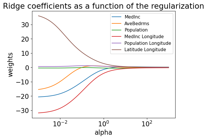
../_images/7074053b90a94b8ec6e8898d8ae9360bc935e8b7e829fd86eb4805d7a8849ea0.png

The coefficients are very close to zero but not exactly zero. That said, they won’t have much impact on prediction.

Regularization learning curves#

plot_learning_curve(Ridge(alpha=0.01), X_train, y_train)
plot_learning_curve(Ridge(alpha=10.0), X_train, y_train)

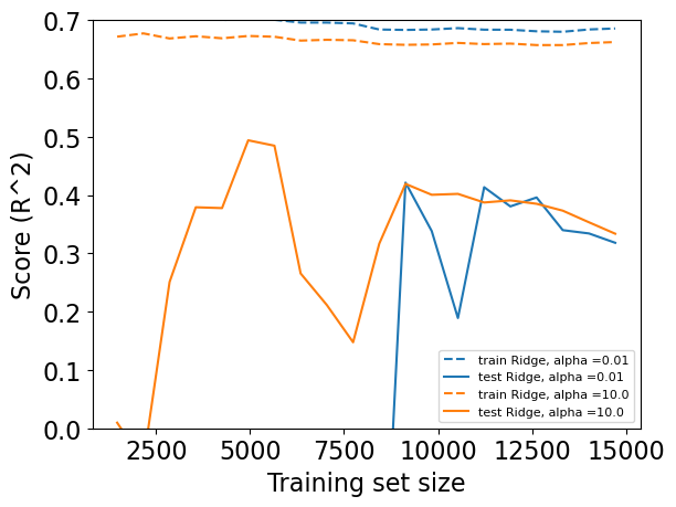
../_images/016c65d8aa215432a7ad8deb6443416b263632ad6eb53b7efe597ef98da05abb.png

As one would expect, the training score is higher than the test score for all dataset sizes
Training score of Ridge with alpha=0.01 > Training score of Ridge with alpha=10 (more regularization)
However, the test score of Ridge with alpha=10 > Test score of Ridge with alpha=0.01 for smaller training sizes.
As more and more data becomes available to the model, both models improve. Ridge with less regularization catches up with ridge with more regularization and actually performs better.

How to pick $\lambda$?#

Theory: as $n$ grows $\lambda$ should be in the range $O(1)$ to $\sqrt{n}$.
Practice: optimize validation set or cross-validation error.
- Almost always decreases the test error.

(Optional) Should we regularize the y-intercept?#

No!
- Why encourage it to be closer to zero? (It could be anywhere.)
- You should be allowed to shift function up/down globally.
Yes!
- Useful for optimization; It makes the solution unique and it easier to compute $w$
Compromise: regularize by a smaller amount than other variables. $$f(w) = \lVert Xw + w_0 - y\rVert^2 + \frac{\lambda_1}{2}\lVert w\rVert^2 + \frac{\lambda_2}{2}w_0^2$$

Some properties of L2-regularization#

Solution $w$ is unique. It has to do with the smoothness of the function.
- We are not going into mathematical details. If interested see slide 20 from CPSC 340.
Almost always improves the validation error.
No collinearity issues.
Less sensitive to changes in $X$.
Gradient descent (optimization algorithm) converges faster (bigger $\lambda$ means fewer iterations). (You’ll learn about Grafient descent in 572.)
Worst case: just set $\lambda$ small and get the same performance

Summary: L2-regularization#

Change the loss function by adding a continuous L2-penalty on the model complexity.
Best parameter $\lambda$ almost already leads to improved validation error.
- L2-regularized least squares is also called “ridge regression”.
- Can be solved as a linear system like least squares.
Some benefits of L2 regularization
- Solution is unique.
- Less sensitive to data.
- Fast.

❓❓ Questions for you (recap)#

iClicker Exercise 6.1#

iClicker cloud join link: https://join.iclicker.com/C0P55

Select all of the following statements which are TRUE.

(A) Introducing L2 regularization to the model means making it less sensitive to changes in $X$.
(B) Introducing L2 regularization to the model can results in worse performance on the training set.
(C) L2 regularization shrinks the weights but all $w_j$s tend to be non-zero.

V’s answers: A, B, C

Break (~5 mins)#

L1 regularization#

An alternative to Ridge (L2-regularization for least squares) is Lasso.
Instead of L0- or L2-norm, regularize with L1-norm.

\[f(w) = \sum_i^n(w^TX_i - y_i)^2 + \lambda\sum_j^d \lvert w_j \lvert\text{ or }\]

\[f(w) = \lVert Xw - y\rVert_2^2 + \lambda \lVert w\rVert_1\]

$\lambda \rightarrow$ regularization strength
$\lVert w\rVert_1 \rightarrow$ L1-norm of $w$
Objective balances getting low error vs. having small values for $w_j$

Similarities with L2-regularization#

L1-regularization $$f(w) = \lVert Xw - y\rVert_2^2 + \lambda \lVert w\rVert_1$$
L2-regularization $$f(w) = \lVert Xw - y\rVert_2^2 + \lambda \lVert w\rVert_2^2$$
Both shrink weights.
Both result in lower validation error.

Do not confuse the L1 loss (absolute loss) with L1-regularization!

Terminology and notation: Ridge and Lasso#

Linear regression model that uses L2 regularization is called Ridge or Tikhonov regularization.
- scikit-learn Ridge
Linear regression model that uses L1 regularization is called Lasso.
- scikit-learn Lasso
class sklearn.linear_model.Lasso(alpha=1.0, fit_intercept=True, normalize=False, precompute=False, copy_X=True, max_iter=1000, tol=0.0001, warm_start=False, positive=False, random_state=None, selection=’cyclic’)

L1-regularization#

The consequence of using L1-norm is that some features are exactly zero, which means that the features are entirely ignored by the model.
This can be considered as a form of feature selection!!
L1-regularization simultaneously regularizes and selects features.
Very fast alternative to search and score methods

Let’s apply Lasso on the California housing data.

X_train.shape

(15480, 44)

from sklearn.linear_model import Lasso

lasso = Lasso().fit(X_train, y_train)
print("Training set score: {:.2f}".format(lasso.score(X_train, y_train)))
print("Test set score: {:.2f}".format(lasso.score(X_test, y_test)))
print("Number of features used:", np.sum(lasso.coef_ != 0))

Training set score: 0.00
Test set score: -0.00
Number of features used: 0

That’s strange. It’s not using any features – like dummy model. It’s underfitting.
Similar to Ridge it also has a regularization hyperparameter alpha.
Let’s decrease it to reduce underfitting.

Let’s examine weight shrinkage for l1 regularization
Lasso loss is not a smooth function.
Slower compared to Ridge.

from numpy.linalg import norm
alphas = [0, 0.0001, 0.01, 0.1, 1]
weight_shrinkage_data = {'alpha':[], '||Xw - y||^2':[], '||w||_1':[], 'intercept':[], 'train score':[], 'test score':[]}

for (i, alpha) in enumerate(alphas): 
    print('alpha: ', alpha)
    l = Lasso(alpha=alpha, max_iter=10000) 
    l.fit(X_train, y_train)
    weight_shrinkage_data['alpha'].append(alpha)
    OLS = np.round(lr_loss_squared(l.coef_, X_train, y_train), 4)
    l1_term = np.round(norm(r.coef_, 1), 4)
    intercept = np.round(l.intercept_, 4)
    weight_shrinkage_data['||Xw - y||^2'].append(OLS)
    weight_shrinkage_data['||w||_1'].append(l1_term)
    weight_shrinkage_data['intercept'].append(intercept)
    weight_shrinkage_data['train score'].append(np.round(l.score(X_train, y_train), 2))
    weight_shrinkage_data['test score'].append(np.round(l.score(X_test, y_test), 2))

alpha:  0

/var/folders/b3/g26r0dcx4b35vf3nk31216hc0000gr/T/ipykernel_27748/2689048393.py:8: UserWarning: With alpha=0, this algorithm does not converge well. You are advised to use the LinearRegression estimator
  l.fit(X_train, y_train)
/Users/kvarada/opt/miniconda3/envs/573/lib/python3.10/site-packages/sklearn/linear_model/_coordinate_descent.py:648: UserWarning: Coordinate descent with no regularization may lead to unexpected results and is discouraged.
  model = cd_fast.enet_coordinate_descent(
/Users/kvarada/opt/miniconda3/envs/573/lib/python3.10/site-packages/sklearn/linear_model/_coordinate_descent.py:648: ConvergenceWarning: Objective did not converge. You might want to increase the number of iterations, check the scale of the features or consider increasing regularisation. Duality gap: 3.394e+03, tolerance: 2.066e+00 Linear regression models with null weight for the l1 regularization term are more efficiently fitted using one of the solvers implemented in sklearn.linear_model.Ridge/RidgeCV instead.
  model = cd_fast.enet_coordinate_descent(

alpha:  0.0001

/Users/kvarada/opt/miniconda3/envs/573/lib/python3.10/site-packages/sklearn/linear_model/_coordinate_descent.py:648: ConvergenceWarning: Objective did not converge. You might want to increase the number of iterations, check the scale of the features or consider increasing regularisation. Duality gap: 1.778e+03, tolerance: 2.066e+00
  model = cd_fast.enet_coordinate_descent(

alpha:  0.01
alpha:  0.1
alpha:  1

pd.DataFrame(weight_shrinkage_data)

	alpha	\|\|Xw - y\|\|^2	\|\|w\|\|_1	intercept	train score	test score
0	0.0000	73398.6742	4.3674	2.0744	0.67	0.52
1	0.0001	73462.0080	4.3674	2.0744	0.67	0.20
2	0.0100	74463.3147	4.3674	2.0744	0.62	0.33
3	0.1000	76723.2012	4.3674	2.0744	0.51	0.48
4	1.0000	87271.1329	4.3674	2.0744	0.00	-0.00

r = Ridge(alpha = 0.1).fit(X_train, y_train)
print("Training set score: {:.2f}".format(r.score(X_train, y_train)))
print("Test set score: {:.2f}".format(r.score(X_test, y_test)))
print("Number of features used:", np.sum(r.coef_ != 0))

Training set score: 0.68
Test set score: 0.62
Number of features used: 44

lasso = Lasso(alpha=0.1, max_iter=10000).fit(X_train, y_train)
print("Training set score: {:.2f}".format(lasso.score(X_train, y_train)))
print("Test set score: {:.2f}".format(lasso.score(X_test, y_test)))
print("Number of features used:", np.sum(lasso.coef_ != 0))

Training set score: 0.51
Test set score: 0.48
Number of features used: 3

In this case we are not really getting better results with Lasso.
In fact, Lasso is not able to do better than linear regression.
Often you might see better scores than Ridge with fewer features.
If alpha is too low, we reduce the effect of overfitting and the results are similar to linear regression.

The weights become smaller and eventually become zero.#

Let’s plot coefficients of Lasso.

alphas = [0, 0.01, 0.1, 1]

plt.figure(figsize=(6, 4))
markers = ['o','*', 'v','^']
lasso_models = {}
for (i, alpha) in enumerate(alphas):
    lasso = Lasso(alpha = alpha, max_iter=10000)
    lasso.fit(X_train, y_train)
    plt.plot(r.coef_, markers[i], markersize=5, label="Lasso alpha="+ str(alpha))
plt.xlabel("Coefficient index")
plt.ylabel("Coefficient magnitude")
plt.hlines(0, 0, len(lasso.coef_))
plt.ylim(-25, 25)
plt.legend(loc="best",fontsize=8);    

/var/folders/b3/g26r0dcx4b35vf3nk31216hc0000gr/T/ipykernel_27748/562400412.py:6: UserWarning: With alpha=0, this algorithm does not converge well. You are advised to use the LinearRegression estimator
  lasso.fit(X_train, y_train)
/Users/kvarada/opt/miniconda3/envs/573/lib/python3.10/site-packages/sklearn/linear_model/_coordinate_descent.py:648: UserWarning: Coordinate descent with no regularization may lead to unexpected results and is discouraged.
  model = cd_fast.enet_coordinate_descent(
/Users/kvarada/opt/miniconda3/envs/573/lib/python3.10/site-packages/sklearn/linear_model/_coordinate_descent.py:648: ConvergenceWarning: Objective did not converge. You might want to increase the number of iterations, check the scale of the features or consider increasing regularisation. Duality gap: 3.394e+03, tolerance: 2.066e+00 Linear regression models with null weight for the l1 regularization term are more efficiently fitted using one of the solvers implemented in sklearn.linear_model.Ridge/RidgeCV instead.
  model = cd_fast.enet_coordinate_descent(

../_images/97aeae6ab39d8fa5c77d468f9ff0a056222901ef551138b70be24f5ca721255b.png

For alpha = 100 most of the coefficients are zero.
With smaller values of alpha we get less and less regularization.

I’m not showing L1 regularization path on our data because it takes too long to run.
But you’re likely to see this type of plots in the context of regularization.

Terminology and notation: Sparsity#

We say a linear function is sparse if most of the coefficients are zero.
Example: Here only 2 out of 8 coefficients are non-zero and so it is a sparse function. $$0x_1 + 0.45 x_2 + 0 x_3 + 0x_4 + 1.2x_5 + 0x_6 + 0x_7 + 0x_8$$
L0- and L1-regularization encourage sparsity.

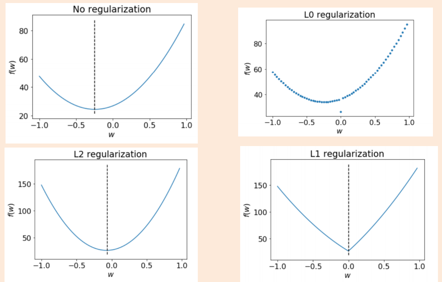
Example: L0 vs. L1 vs. L2#

Consider problem where 3 vectors can get minimum training error:

\[\begin{split}w^1 = \begin{bmatrix}100 \\0.02\end{bmatrix}, w^2 = \begin{bmatrix}100 \\0\end{bmatrix}, w^3 = \begin{bmatrix}99.99 \\0.02\end{bmatrix}\end{split}\]

Without regularization, we could choose any of these 3.
We are assuming that all have the same error, so regularization will “break tie”.
Which one would you choose with each of L0, L1, L2 regularization?

Which one would you choose with L0 regularization?#

\[\begin{split}w^1 = \begin{bmatrix}100 \\-0.02\end{bmatrix}, w^2 = \begin{bmatrix}100 \\0\end{bmatrix}, w^3 = \begin{bmatrix}99.99 \\0.02\end{bmatrix}\end{split}\]

What are the L0 norms of different weight vectors?
- $\lVert w^1\rVert_0 = 2$
- $\lVert w^2\rVert_0 = 1$
- $\lVert w^3\rVert_0 = 2$
L0 regularization would choose $w^2$.

Which one would you choose with L1 regularization?#

\[\begin{split}w^1 = \begin{bmatrix}100 \\0.02\end{bmatrix}, w^2 = \begin{bmatrix}100 \\0\end{bmatrix}, w^3 = \begin{bmatrix}99.99 \\0.02\end{bmatrix}\end{split}\]

What are the L1 norms of different weight vectors?
- $\lVert w^1\rVert_1 = 100.02$
- $\lVert w^2\rVert_1 = 100$
- $\lVert w^3\rVert_1 = 100.01$

L1-regularization would pick $w^2$
L1-regularization focuses on decreasing all $w_j$ until they are 0.

Which one would you choose with L2 regularization?#

\[\begin{split}w^1 = \begin{bmatrix}100 \\0.02\end{bmatrix}, w^2 = \begin{bmatrix}100 \\0\end{bmatrix}, w^3 = \begin{bmatrix}99.99 \\0.02\end{bmatrix}\end{split}\]

What are the L2 norms of different weight vectors?
- $\lVert w^1\rVert_2^2 = (100)^2 + (0.02)^2 = 10000.0004$
- $\lVert w^2\rVert_2^2 = (100)^2 = 10000$
- $\lVert w^3\rVert_2^2 = (99.99)^2 + (0.02)^2 = 9998.0005$

L2-regularization would pick $w^3$
L2-regularization focuses on decreasing largest $w_j$ smaller

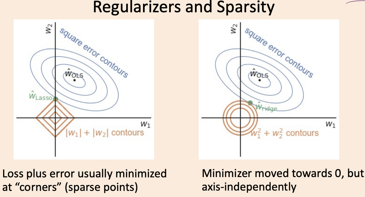
(Optional) Sparsity and Regularization#

Minimizing $\lVert Xw - y\rVert_2^2 + \lambda \lVert w\rVert_2^2$ is equivalent to minimizing $\lVert Xw - y\rVert_2^2$ subject to the constraint that $\lVert w\rVert_2^2 \leq t(\delta)$

Source

Sparsity and Regularization (with d=1)#

Some properties of L1 regularization#

Almost always improves the validation error.
Can learn with exponential number of irrelevant features.
Less sensitive to changes in $X$.
The solution is not unique. (If interested in more explanation on this, see slide 43 in this slide deck.)

Feature selection using L1 regularization#

Feature selection methods we have seen so far:
- RFE
- Search and score with L0-regularization (e.g., forward search)
An effective way of feature selection: L1-regularization

from sklearn.ensemble import RandomForestRegressor
from sklearn.feature_selection import SelectFromModel
from sklearn.linear_model import Lasso, LassoCV

housing = fetch_california_housing(as_frame=True)
X = housing["data"]
y = housing["target"]
X_train, X_test, y_train, y_test = train_test_split(X, y, random_state=0)
pipe_l1_rf = make_pipeline(
    StandardScaler(),
    SelectFromModel(Lasso(alpha=0.01, max_iter=100000)),
    RandomForestRegressor(),
)

X.shape

(20640, 8)

pipe_l1_rf.fit(X_train, y_train)
pipe_l1_rf.score(X_train, y_train)

0.9731789734697873

print("Training set score: {:.2f}".format(pipe_l1_rf.score(X_train, y_train)))
print("Test set score: {:.2f}".format(pipe_l1_rf.score(X_test, y_test)))

Training set score: 0.97
Test set score: 0.79

print(
    "Number of features used:",
    np.sum(pipe_l1_rf.named_steps["selectfrommodel"].estimator_.coef_ != 0),
)

Number of features used: 7

Regularized models for classification#

Regularized logistic regression#

Regularization is not limited to least squares.
We can add L1 and L2 penalty terms in other loss functions as well.
Let’s look at logistic regression with L1- and L2-regularization.

from sklearn.datasets import load_breast_cancer

breast_cancer = load_breast_cancer()
# print(breast_cancer.keys())
# print(breast_cancer.DESCR)

breast_cancer_df = pd.DataFrame(breast_cancer.data, columns=breast_cancer.feature_names)
breast_cancer_df["target"] = breast_cancer.target
train_df, test_df = train_test_split(breast_cancer_df, test_size=0.2, random_state=2)

X_train, y_train = train_df.drop(columns=["target"]), train_df["target"]
X_test, y_test = test_df.drop(columns=["target"]), test_df["target"]

X_train.head()

	mean radius	mean texture	mean perimeter	mean area	mean smoothness	mean compactness	mean concavity	mean concave points	mean symmetry	mean fractal dimension	...	worst radius	worst texture	worst perimeter	worst area	worst smoothness	worst compactness	worst concavity	worst concave points	worst symmetry	worst fractal dimension
560	14.05	27.15	91.38	600.4	0.09929	0.11260	0.04462	0.04304	0.1537	0.06171	...	15.30	33.17	100.20	706.7	0.1241	0.22640	0.1326	0.10480	0.2250	0.08321
428	11.13	16.62	70.47	381.1	0.08151	0.03834	0.01369	0.01370	0.1511	0.06148	...	11.68	20.29	74.35	421.1	0.1030	0.06219	0.0458	0.04044	0.2383	0.07083
198	19.18	22.49	127.50	1148.0	0.08523	0.14280	0.11140	0.06772	0.1767	0.05529	...	23.36	32.06	166.40	1688.0	0.1322	0.56010	0.3865	0.17080	0.3193	0.09221
203	13.81	23.75	91.56	597.8	0.13230	0.17680	0.15580	0.09176	0.2251	0.07421	...	19.20	41.85	128.50	1153.0	0.2226	0.52090	0.4646	0.20130	0.4432	0.10860
41	10.95	21.35	71.90	371.1	0.12270	0.12180	0.10440	0.05669	0.1895	0.06870	...	12.84	35.34	87.22	514.0	0.1909	0.26980	0.4023	0.14240	0.2964	0.09606

5 rows × 30 columns

y_train.value_counts(normalize=True)

1    0.632967
0    0.367033
Name: target, dtype: float64

from sklearn.metrics import f1_score, make_scorer, recall_score

custom_scorer = make_scorer(
    f1_score, pos_label=0
)  # note the syntax to change the positive label for f1 score
scoring_metric = custom_scorer

results_classification = {}

Let’s try DummyClassifier

dummy = DummyClassifier()
results_classification["dummy"] = mean_std_cross_val_scores(
    dummy,
    X_train,
    y_train,
    return_train_score=True,
    scoring=scoring_metric,
)
pd.DataFrame(results_classification)

	dummy
fit_time	0.000 (+/- 0.001)
score_time	0.000 (+/- 0.000)
test_score	0.000 (+/- 0.000)
train_score	0.000 (+/- 0.000)

In sklearn, by default logistic regression uses L2 regularization.
The C hyperparameter decides the strength of regularization.
Unfortunately, interpretation of C is inverse of lambda.

pipe_lgr_l2 = make_pipeline(StandardScaler(), LogisticRegression())
results_classification["Logistic Regression L2"] = mean_std_cross_val_scores(
    pipe_lgr_l2, X_train, y_train, return_train_score=True, scoring=scoring_metric
)

pd.DataFrame(results_classification)

	dummy	Logistic Regression L2
fit_time	0.000 (+/- 0.001)	0.005 (+/- 0.002)
score_time	0.000 (+/- 0.000)	0.001 (+/- 0.000)
test_score	0.000 (+/- 0.000)	0.970 (+/- 0.011)
train_score	0.000 (+/- 0.000)	0.985 (+/- 0.005)

Weights are small but all of them are non-zero.

pipe_lgr_l2.fit(X_train, y_train)
l2_coefs = pipe_lgr_l2.named_steps["logisticregression"].coef_.flatten()
df = pd.DataFrame(l2_coefs, index=X_train.columns, columns=["l2_coefs"])
df

	l2_coefs
mean radius	-0.539854
mean texture	-0.252141
mean perimeter	-0.494560
mean area	-0.610451
mean smoothness	-0.174066
mean compactness	0.577983
mean concavity	-0.658777
mean concave points	-0.980244
mean symmetry	0.119974
mean fractal dimension	0.406479
radius error	-1.247956
texture error	-0.103258
perimeter error	-0.731201
area error	-0.931584
smoothness error	-0.230991
compactness error	0.614317
concavity error	-0.032318
concave points error	-0.206376
symmetry error	0.272883
fractal dimension error	0.739561
worst radius	-1.040150
worst texture	-1.096207
worst perimeter	-0.885489
worst area	-1.026863
worst smoothness	-0.927290
worst compactness	-0.075403
worst concavity	-0.766568
worst concave points	-0.732966
worst symmetry	-0.669925
worst fractal dimension	-0.520939

Let’s try logistic regression with L1 regularization.
Note that I’m using a different solver (optimizer) here because not all solvers support L1-regularization.

pipe_lgr_l1 = make_pipeline(
    StandardScaler(), LogisticRegression(solver="liblinear", penalty="l1")
)
results_classification["Logistic Regression L1"] = mean_std_cross_val_scores(
    pipe_lgr_l1, X_train, y_train, return_train_score=True, scoring=scoring_metric
)

pd.DataFrame(results_classification)

	dummy	Logistic Regression L2	Logistic Regression L1
fit_time	0.000 (+/- 0.001)	0.005 (+/- 0.002)	0.003 (+/- 0.001)
score_time	0.000 (+/- 0.000)	0.001 (+/- 0.000)	0.001 (+/- 0.000)
test_score	0.000 (+/- 0.000)	0.970 (+/- 0.011)	0.967 (+/- 0.007)
train_score	0.000 (+/- 0.000)	0.985 (+/- 0.005)	0.985 (+/- 0.005)

The scores are more or less the same.

But L1 regularization is carrying out feature selection; Many coefficients are 0.
Similar scores with less features! More interpretable model!

pipe_lgr_l1.fit(X_train, y_train)
l1_coefs = pipe_lgr_l1.named_steps["logisticregression"].coef_.flatten()
df["l1_coef"] = l1_coefs
df

	l2_coefs	l1_coef
mean radius	-0.539854	0.000000
mean texture	-0.252141	0.000000
mean perimeter	-0.494560	0.000000
mean area	-0.610451	0.000000
mean smoothness	-0.174066	0.000000
mean compactness	0.577983	0.000000
mean concavity	-0.658777	0.000000
mean concave points	-0.980244	-1.337092
mean symmetry	0.119974	0.000000
mean fractal dimension	0.406479	0.271158
radius error	-1.247956	-2.007079
texture error	-0.103258	0.000000
perimeter error	-0.731201	0.000000
area error	-0.931584	0.000000
smoothness error	-0.230991	-0.127449
compactness error	0.614317	0.537477
concavity error	-0.032318	0.000000
concave points error	-0.206376	0.000000
symmetry error	0.272883	0.000000
fractal dimension error	0.739561	0.227465
worst radius	-1.040150	-1.382266
worst texture	-1.096207	-1.372887
worst perimeter	-0.885489	-0.419092
worst area	-1.026863	-3.613997
worst smoothness	-0.927290	-0.984068
worst compactness	-0.075403	0.000000
worst concavity	-0.766568	-1.011790
worst concave points	-0.732966	-0.660896
worst symmetry	-0.669925	-0.299326
worst fractal dimension	-0.520939	0.000000

We can also carry out feature selection using L1 regularization and pass selected features to another model.

from lightgbm.sklearn import LGBMClassifier

pipe_lgr_lgbm = make_pipeline(
    StandardScaler(),
    SelectFromModel(LogisticRegression(solver="liblinear", penalty="l1")),
    LGBMClassifier(),
)

results_classification["L1 + LGBM"] = mean_std_cross_val_scores(
    pipe_lgr_lgbm,
    X_train,
    y_train,
    return_train_score=True,
    scoring=scoring_metric,
)
pd.DataFrame(results_classification)

	dummy	Logistic Regression L2	Logistic Regression L1	L1 + LGBM
fit_time	0.000 (+/- 0.001)	0.005 (+/- 0.002)	0.003 (+/- 0.001)	0.151 (+/- 0.015)
score_time	0.000 (+/- 0.000)	0.001 (+/- 0.000)	0.001 (+/- 0.000)	0.001 (+/- 0.000)
test_score	0.000 (+/- 0.000)	0.970 (+/- 0.011)	0.967 (+/- 0.007)	0.957 (+/- 0.034)
train_score	0.000 (+/- 0.000)	0.985 (+/- 0.005)	0.985 (+/- 0.005)	1.000 (+/- 0.000)

The score went down a bit this case. But this might help in some other cases.
The resulting model is using L1 selected features only.

How to use regularization with `scikit-learn`: some examples#

Regression
- Least squares with L2-regularization: Ridge
- Least squares with L1-regularization: Lasso
- Least squares with L1- and L2-regularization: ElasticNet
- SVR ($\epsilon$-insensitive loss function)
  - epsilon = 0 gives us KernelRidge model (least squares with RBF)
Classification
- SVC (supports L2-regularization)
- LogisticRegression (support L1 and L2 with different solvers)
penalty{‘l1’, ‘l2’, ‘elasticnet’, ‘none’}, default=’l2’ Used to specify the norm used in the penalization. The ‘newton-cg’, ‘sag’ and ‘lbfgs’ solvers support only l2 penalties. ‘elasticnet’ is only supported by the ‘saga’ solver. If ‘none’ (not supported by the liblinear solver), no regularization is applied.

Interpretations of coefficients of regularized linear models should always be taken with a grain of salt.
With different values of the regularization parameter, sometimes even the signs of the coefficients might change!!

Regularization: scaling and collinearity#

Regularization and scaling#

It doesn’t matter for decision trees or naive Bayes.
- They only look at one feature at a time.
It doesn’t matter for least squares:
- $w_j*(100 mL)$ gives the same model as $w_j*(0.1 L)$ with a different $w_j$
It matters for $k$-nearest neighbours:
- Distance will be affected more by large features than small features.
It matters for regularized least squares:
- Penalizing $w_j^2$ means different things if features $j$ are on different scales
- Penalizing $w_j$ means different things if features $j$ are on different scales

Collinearity and regularization#

If you have colinear features, the weights would go crazy with regular linear regression.
With L2 regularization: The weight will be equally distributed among all collinear features because the solution is unique.
- Example: suppose we have three identical features with a total weight of 1
- The weight will be distributed as 1/3, 1/3, 1/3 among the features.
With L1 regularization: The weight will not be equally distributed; the solution is not unique.
- Example: suppose we have three identical features with a total weight of 1
- The weight could be distributed in many different ways
- For example, 1/2, 1/4, 1/4 or 1.0, 0, 0 or 1/2, 1/2, 0 and so on …

Elastic nets#

Combine good properties from both worlds

\[f(w) = \lVert Xw - y\rVert_2^2 + \lambda(\alpha\lVert w\rVert_1 + (1-\alpha)\lVert w\rVert_2^2 ) \]

$\lambda$ control the strength of regularization
$\alpha$ controls the amount of sparsity and smoothness
L1 promotes sparsity and the L2 promotes smoothness.
The functional is strictly convex: the solution is unique.
No collinearity problem
- A whole group of correlated variables is selected rather than just one variable in the group.

You can use elastic nets using sklearn’s ElasticNet.

Summary: L* regularization#

L0-regularization (AIC, BIC, Mallow’s Cp, Adjusted R2, ANOVA): More on this is DSCi 562
- Adds penalty on the number of non-zeros to select features.

\[f(w) = \lVert Xw - y\rVert_2^2 + \lambda\lVert w\rVert_0\]

L2-regularization (ridge regression):
- Adding penalty on the L2-norm of $w$ to decrease overfitting: $$f(w) = \lVert Xw - y\rVert_2^2 + \lambda \lVert w\rVert_2^2$$
L1-regularization (lasso regression):
- Adding penalty on the L1-norm decreases overfitting and selects features: $$f(w) = \lVert Xw - y\rVert_2^2 + \lambda \lVert w\rVert_1$$

Interpretations of coefficients of linear models should always be taken with a grain of salt
- Regularizing a model might change the sign of the coefficients.
Un-regularized linear regression: not affected by scaling
L1 or L2-regularized linear regression: both affected by scaling (and it’s usually a good idea)

Lecture 6: L2- and L1-Regularization

Contents

Lecture 6: L2- and L1-Regularization#

Imports#

Learning outcomes#

Recap#

Idea of regularization: Pick the line/hyperplane with smaller slope#

How to quantify model complexity?#

L0-regularization#

L2-regularization#

sklearn’s Ridge or L2 regularization#

Example: L2-Regularization “Shrinking”#

The weights become smaller but do not become zero#

Regularization path#

Regularization learning curves#

How to pick \(\lambda\)?#

(Optional) Should we regularize the y-intercept?#

Some properties of L2-regularization#

Summary: L2-regularization#

❓❓ Questions for you (recap)#

iClicker Exercise 6.1#

Break (~5 mins)#

L1 regularization#

Similarities with L2-regularization#

Terminology and notation: Ridge and Lasso#

L1-regularization#

The weights become smaller and eventually become zero.#

Terminology and notation: Sparsity#

Example: L0 vs. L1 vs. L2#

Which one would you choose with L0 regularization?#

Which one would you choose with L1 regularization?#

Which one would you choose with L2 regularization?#

(Optional) Sparsity and Regularization#

Sparsity and Regularization (with d=1)#

Some properties of L1 regularization#

Feature selection using L1 regularization#

Regularized models for classification#

Regularized logistic regression#

How to use regularization with scikit-learn: some examples#

Regularization: scaling and collinearity#

Regularization and scaling#

Collinearity and regularization#

Elastic nets#

Summary: L* regularization#

`sklearn`’s `Ridge` or L2 regularization#

How to use regularization with `scikit-learn`: some examples#