Introduction to simplerfit • simplerfit

library(simplerfit)

Brief Introduction

Simplerfit is a package that will help reduce effort in each section of a model building pipeline. There are five functions that are included in this R package which are described in more detail below. Seasoned and amateur data scientists’ can use this package in their pipelines to make their tasks more efficient.

This document introduces you to simplerfit’s functions and how to use them.

Data

To explore the basic functionality of simplerfit we use the dataset gapminder. If you want to visualize the data, before going through the functions, use the code below to load it.

# load gapminder dataset
gapminder <- gapminder::gapminder
head(gapminder)
#> # A tibble: 6 × 6
#>   country     continent  year lifeExp      pop gdpPercap
#>   <fct>       <fct>     <int>   <dbl>    <int>     <dbl>
#> 1 Afghanistan Asia       1952    28.8  8425333      779.
#> 2 Afghanistan Asia       1957    30.3  9240934      821.
#> 3 Afghanistan Asia       1962    32.0 10267083      853.
#> 4 Afghanistan Asia       1967    34.0 11537966      836.
#> 5 Afghanistan Asia       1972    36.1 13079460      740.
#> 6 Afghanistan Asia       1977    38.4 14880372      786.

Function Demonstration

Cleaning the dataframe

The cleaner function does the basic cleaning of a raw data-frame by removing the empty rows, stripping extra white spaces in the data and converting the column names to lower case.

clean_df <- clean_data(gapminder)
head(clean_df)
#> # A tibble: 6 × 6
#>   country     continent  year lifeexp      pop gdppercap
#>   <fct>       <fct>     <int>   <dbl>    <int>     <dbl>
#> 1 Afghanistan Asia       1952    28.8  8425333      779.
#> 2 Afghanistan Asia       1957    30.3  9240934      821.
#> 3 Afghanistan Asia       1962    32.0 10267083      853.
#> 4 Afghanistan Asia       1967    34.0 11537966      836.
#> 5 Afghanistan Asia       1972    36.1 13079460      740.
#> 6 Afghanistan Asia       1977    38.4 14880372      786.

EDA

The functions take in the cleaned data set to create a correlation plot and a distribution plot.

plot_corr(clean_df, corr = 'pearson', pair_cols=c('lifeexp', 'pop', 'gdppercap'))
#> Registered S3 method overwritten by 'GGally':
#>   method from   
#>   +.gg   ggplot2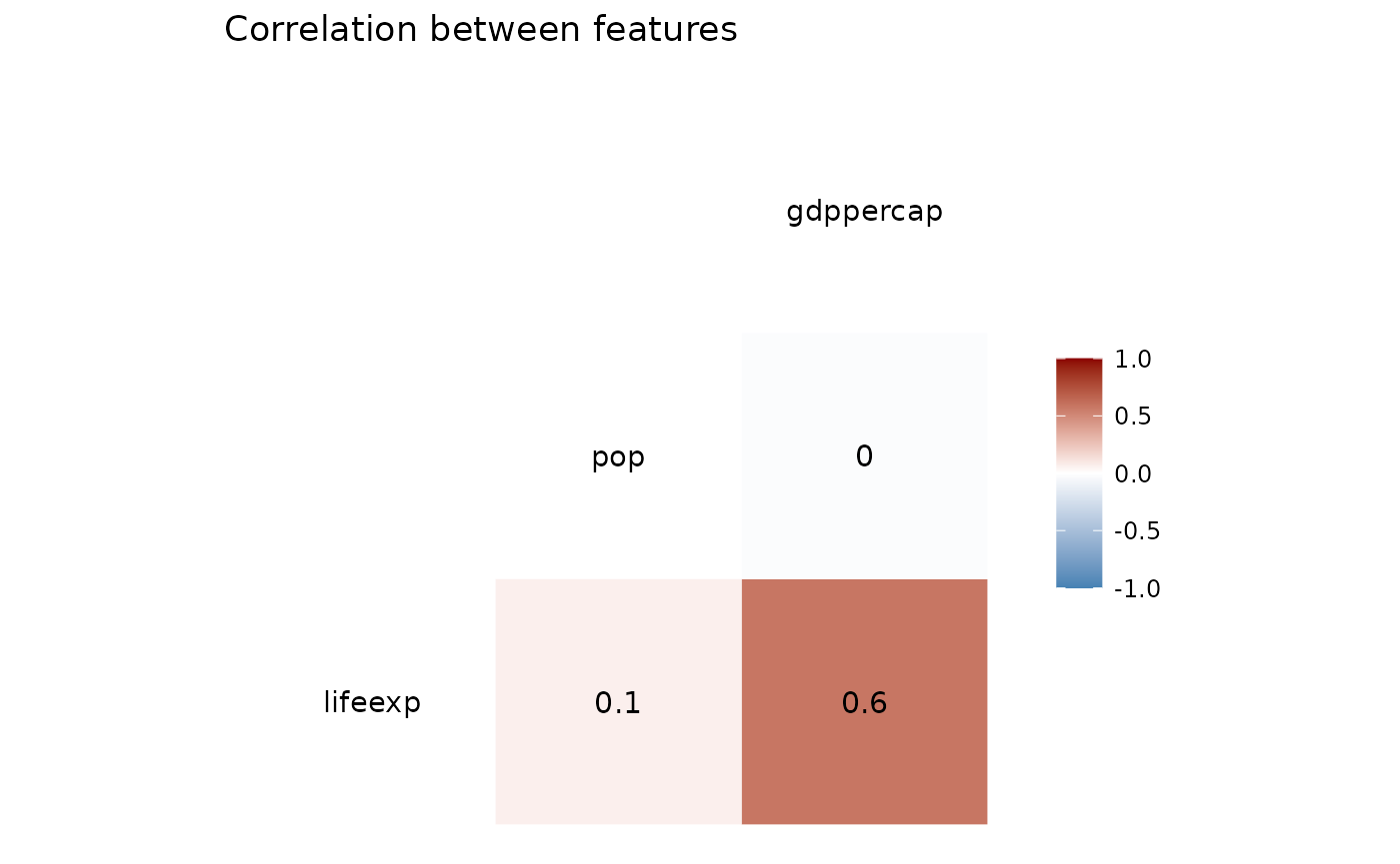


plot_distributions(clean_df, bins = 30, hist_cols=c("gdppercap"))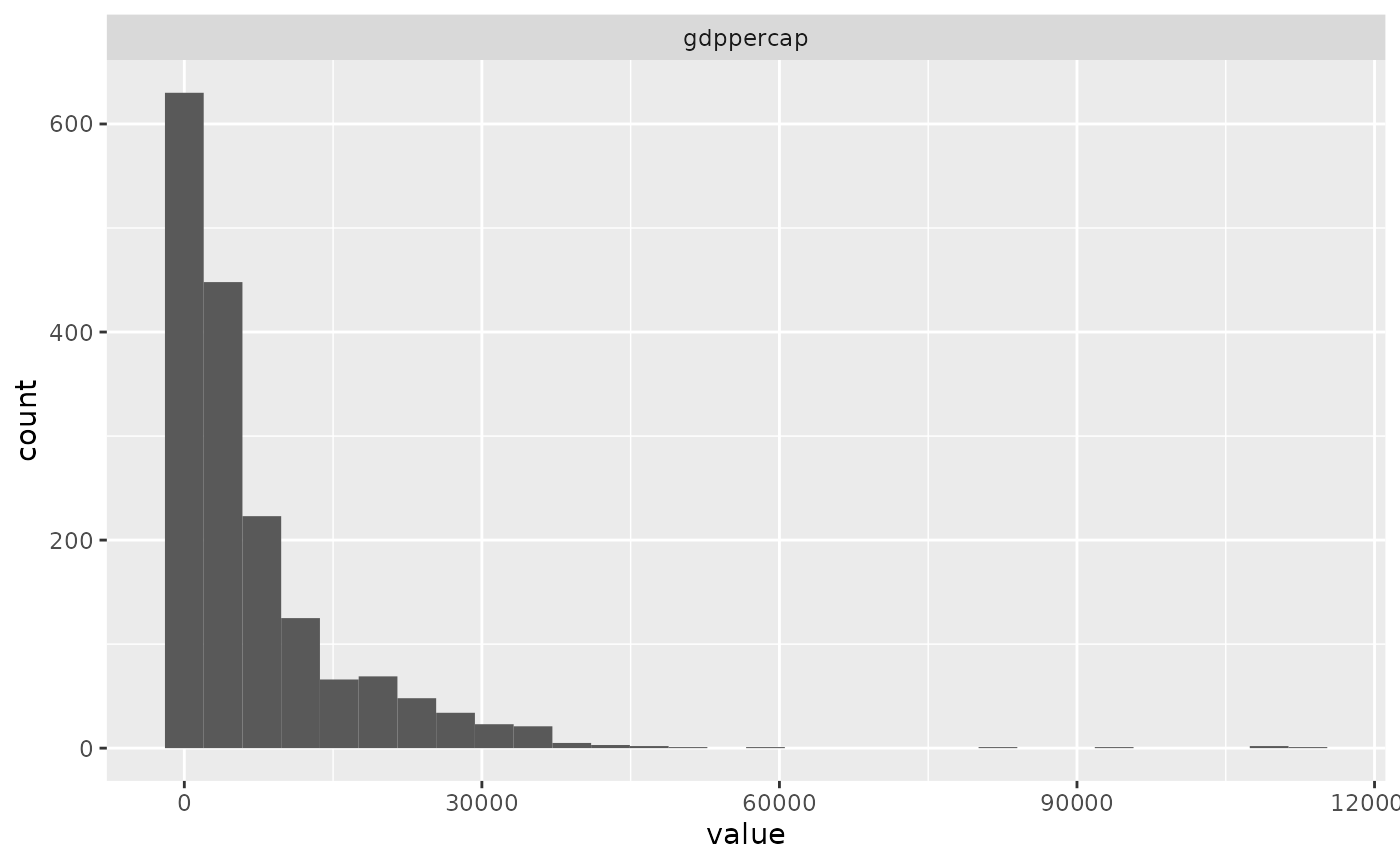

Regression

If the problem is of a regression nature, the RMSE scores of dummy regressor, linear regressor and ridge are compared

suppressWarnings(fit_regressor(clean_df, 
              target_col="gdppercap", 
              numeric_feats=c("year", "lifeexp", "pop"), 
              categorical_feats <- c("continent"), 
              cv =5))
#> Loading required package: ggplot2
#> Loading required package: lattice
#> t=100, m=5
#> t=200, m=6
#> t=300, m=6
#> t=400, m=6
#> t=500, m=5
#> t=600, m=5
#> t=700, m=5
#> t=800, m=6
#> t=900, m=5
#> t=100, m=7
#> t=200, m=6
#> t=300, m=5
#> t=400, m=6
#> t=500, m=5
#> t=600, m=7
#> t=700, m=6
#> t=800, m=6
#> t=900, m=6
#> t=100, m=6
#> t=200, m=6
#> t=300, m=5
#> t=400, m=7
#> t=500, m=4
#> t=600, m=7
#> t=700, m=6
#> t=800, m=5
#> t=900, m=5
#> t=100, m=6
#> t=200, m=5
#> t=300, m=6
#> t=400, m=6
#> t=500, m=4
#> t=600, m=6
#> t=700, m=6
#> t=800, m=4
#> t=900, m=4
#> t=100, m=4
#> t=200, m=6
#> t=300, m=5
#> t=400, m=5
#> t=500, m=4
#> t=600, m=5
#> t=700, m=3
#> t=800, m=4
#> t=900, m=6
#> t=100, m=5
#> t=200, m=6
#> t=300, m=6
#> t=400, m=6
#> t=500, m=6
#> t=600, m=5
#> t=700, m=6
#> t=800, m=6
#> t=900, m=6
#>              models  Rsquared     RMSE
#> 1   Dummy regressor       NaN 9758.116
#> 2 Linear regression 0.4021298 7596.120
#> 3             Ridge 0.3774341 7768.282

Classification

If the problem is of a classification nature, the accuracy scores of dummy classifier and logistic regression are compared

clean_df <- clean_df |> dplyr::filter(continent=="Asia" | continent=="Europe")
clean_df$country <- as.character(clean_df$country)
clean_df$continent <- as.character(clean_df$continent)
clean_df$year <- as.numeric(clean_df$year)
clean_df$pop <- as.numeric(clean_df$pop)

suppressWarnings(fit_classifier(clean_df, 
               target_col = 'continent', 
               numeric_feats = list('gdppercap'), 
               categorical_feats = list('country'), 
               cv = 5))
#>   dummy_classifier logistic_regression
#> 1        0.5238062                   1