Lecture 4 - Markov Chain Monte Carlo, Stan, and Complex Bayesian Models

Lecture 4 - Markov Chain Monte Carlo, `Stan`, and Complex Bayesian Models#

Today’s Learning Objectives#

Illustrate the steps to build a likelihood in a Bayesian design.
Explore a complex dataset involving categorical, count, and continuous variables.
Apply a Bayesian model design with the proper random variables (Normal, Gamma, and Poisson).
Explain the general procedure of Markov Chain Monte Carlo (MCMC).
Practice computational Bayesian inference via Stan.
Draw inferential conclusions from our posterior distribution of parameters.

Loading `R` Packages#

options(repr.matrix.max.rows = 6, repr.matrix.max.cols = 10)
library(tidyverse)
library(janitor)
library(cowplot)
library(rstan)
library(bayesplot)
library(wesanderson)

Previously…#

We have explored the Bayesian framework on a conceptual level at the beginning of the course. Then, we got familiar with the Bayes’ rule via probability theory. Recall the Bayes’ rule as one of the most powerful components in Bayesian analysis. By applying this rule, we solved a foundational model called the Beta-Binomial in which we combine two random variables via our likelihood and prior distribution. Moreover, we explored the Gamma-Poisson model during lab time.

Nonetheless, real-life problems are not theoretically well behaved as the Beta-Binomial and Gamma Poisson cases. Moreover, complex data will require even more diverse distributions to design our Bayesian model. Hence, the analytical application of the Bayes’ rule will not be possible for a nice exact posterior distribution.

Important

Let us not worry! Stan will come in handy given this issue via MCMC to obtain an approximate posterior distribution.

1. The Big Idea#

Let us recall the big idea of Bayesian modelling. It involves these steps:

Question: Pose a scientific question.
Design: Formulate variables and create a probabilistic model for them. Prior knowledge is included here!
Infer: Get posterior samples from the conditional distribution of any variable you want to infer, given your observed data and prior knowledge.
Check: Make sure the “samples” are actually from your posterior (these are model diagnostics, to be covered later!)
Analyze: Use your samples to compute summaries: mean, maximum a posteriori (MAP), variance, posterior credible intervals, etc.

The scientific question can involve inferential and/or predictive inquiries:

Inferential: Using observed data $Y$ to infer latent variable $\theta$.
Predictive: Using observed data $Y$ to predict future data $Y'$.

We already discussed their differences in Lecture 3 - Bayesian Statistics in Action: The Beta-Binomial Model our via some examples. Now, let us think generatively!

1.1. To Design the Model, Think Generatively!#

Ultimately, our model is an abstraction of a complex system involving different parameters of interest. Suppose we have $d$ parameters $\theta_1, \dots, \theta_d$. Mathematically, these $d$ parameters can be put in a vector as follows:

\[\Theta = (\theta_1, \dots, \theta_d)^T.\]

Note our Bayesian model is a big joint probability distribution $P(Y, Y', \Theta)$ over:

Things we will see. Our observations $Y$.
Things we have to infer: Unobserved parameters $\Theta$ and predicted observations $Y'$. This is why the posterior distribution of $\Theta$ is key!

We already had a first inferential approach (analytically speaking!) via the Beta-Binomial model in Lecture 3 - Bayesian Statistics in Action: The Beta-Binomial Model.

Now, it is much more intuitive to design a couple of steps that generate parameters and synthetic data:

First, generate $\Theta$ from the prior $P(\Theta)$.
Then, generate observations $Y$, $Y'$ given $\Theta$ from the likelihood $P(Y,Y'|\Theta)$.

Attention

We are basically applying the law of conditioning

\[P(Y,Y',\Theta) = P(Y,Y'|\Theta)P(\Theta).\]

We will start with the likelihood. This function involves formulating certain variables. It is the core part of the model design! Then, we can establish the prior distributions for our parameters of interest within $\Theta$ (the likelihood will be of a big help here).

Important

This whole thing is a story of how our data were created.

So far in lab1, we only used our generative Monte Carlo models to simulate synthetic data given some fixed parameters. Nonetheless, we did not incorporate any observed data. In lab2, we will need to include observed data.

1.2. Constructing the Likelihood#

To construct the distribution of the model parameters in $\Theta$ conditioned on the observed data $Y$ (i.e., the likelihood), we need to follow these steps:

Step 1: Formulate all data variables - type (integer, real, categorical, etc.) and support (positive, nonnegative, binary, etc.).
Step 2: Figure out which variables we will take as fixed covariates, which will be randomly generated, and how they are related.
Step 3: Pick a distribution with the right support/type/dependencies. The support refers to a proper range of plausible values. Usually, the distribution will have some UNKNOWN PARAMETERS - those will need a prior!

2. The Bikeshare Data#

Let us recheck the bikeshare data. This is a complex case in which we have variables of different types.

Description: Hourly record of the number of bike trips in Washington, DC in 2011/2012.
Source: 2011/12 Capital Bikeshare Data.
Variables: date, hour, holiday/weekend/workday, weather, temperature, number of trips.

Main statistical inquiries

Suppose we are interested in the following inferential inquiries:

How are temperature and weather associated with the mean number of trips?
Specifically, does the mean number of trips vary by the type of weather along with temperature?
How can we quantify this variation?

Let us start with in-class questions.

Exercise 11

Let us retake DSCI 562 topics under a frequentist approach; what regression modelling can approach the above inquiries?

A. A generalized linear model (GLM) such as Multinomial regression.

B. A GLM such as Ordinal Logistic regression.

C. A GLM such as Poisson regression.

D. Ordinary Least-squares (OLS).

2.1. Data Wrangling#

The data frame bikeshare_data contains sixteen different variables. For the sake of our example and inquiries, we will use a small subset of them.

bikeshare_data <- read_csv("../data/bikeshare_hourly.csv", show_col_types = FALSE)
bikeshare_data

A spec_tbl_df: 17379 × 17
instant	dteday	season	yr	mnth	⋯	hum	windspeed	casual	registered	cnt
<dbl>	<date>	<dbl>	<dbl>	<dbl>	⋯	<dbl>	<dbl>	<dbl>	<dbl>	<dbl>
1	2011-01-01	1	0	1	⋯	0.81	0	3	13	16
2	2011-01-01	1	0	1	⋯	0.80	0	8	32	40
3	2011-01-01	1	0	1	⋯	0.80	0	5	27	32
⋮	⋮	⋮	⋮	⋮	⋱	⋮	⋮	⋮	⋮	⋮
17377	2012-12-31	1	1	12	⋯	0.60	0.1642	7	83	90
17378	2012-12-31	1	1	12	⋯	0.56	0.1343	13	48	61
17379	2012-12-31	1	1	12	⋯	0.65	0.1343	12	37	49

We quickly wrangle our data, select, and rename the three variables of interest:

weather: A categorical variable indicating the overall weather situation. It is coded as:
- 1: Clear, Few clouds, Partly cloudy.
- 2: Mist + Cloudy, Mist + Broken clouds, Mist + Few clouds, Mist.
- 3: Light Snow, Light Rain + Thunderstorm + Scattered clouds, Light Rain + Scattered clouds.
temp: Temperature in Celsius degrees. The values are multiplied times 41 since they were normalized in the original dataset with the maximum value (you can check the Readme.txt). It is a continuous variable.
ride_count: Count of total rental bikes, including casual and registered. It is an integer-type variable.

Attention

Originally, there was a category 4 (Heavy Rain + Ice Pallets + Thunderstorm + Mist, Snow + Fog) in weather. Nonetheless, only three rows contained this category. Hence, they were removed, yielding 17376 rows in total to be used.

bikeshare_data <- bikeshare_data |>
  select(weathersit, temp, cnt) |>
  mutate(temp = temp * 41) |>
  filter(weathersit < 4)
colnames(bikeshare_data) <- c("weather", "temp", "ride_count")
bikeshare_data

A tibble: 17376 × 3
weather	temp	ride_count
<dbl>	<dbl>	<dbl>
1	9.84	16
1	9.02	40
1	9.02	32
⋮	⋮	⋮
1	10.66	90
1	10.66	61
1	10.66	49

nrow(bikeshare_data)

17376

2.2. Exploratory Data Analysis#

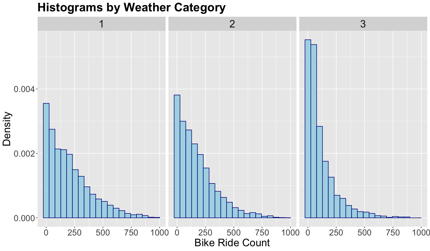
There is a reason why the exploratory data analysis (EDA) is extremely helpful in Bayesian modelling. We might wonder, how do ride counts behave by weather category?

Firstly, let us plot histograms of ride_count by category in weather. Note the $y$-axis is adjusted with after_stat(density) since category 3 is present in fewer rows in bikeshare_data

bikeshare_data |> 
  tabyl(weather) |>
  adorn_pct_formatting()

A tabyl: 3 × 3
weather	n	percent
<dbl>	<dbl>	<chr>
1	11413	65.7%
2	4544	26.2%
3	1419	8.2%

options(repr.plot.height = 7, repr.plot.width = 12)

bikeshare_data_hist <- ggplot(bikeshare_data, aes(
  x = ride_count, y = after_stat(density)
)) +
  geom_histogram(bins = 20, color = "darkblue", fill = "lightblue") +
  labs(y = "Density", x = "Bike Ride Count", fill = "") +
  ggtitle("Histograms by Weather Category") +
  theme(
    plot.title = element_text(size = 24, face = "bold"),
    axis.text.x = element_text(size = 17, angle = 0),
    axis.text.y = element_text(size = 17, angle = 0),
    axis.title = element_text(size = 21),
    strip.text.x = element_text(size = 21)
  ) +
  facet_grid(. ~ as.factor(weather))

bikeshare_data_hist

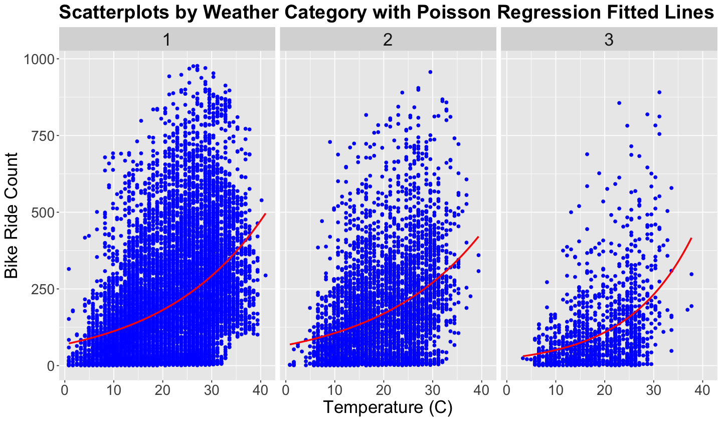
../_images/7baebf9d188c65737ce6999236e3c87d772d9049476fe0a3d97500c538cd6242.png

Now, how can we plot the relationship between ride_count and temp by weather category? Let us create scatterplots of temp versus ride_count by weather category.

Hint

Identifying patterns with count versus continuous data is not straightforward. How about if we apply what we learned in DSCI 562? Let us fit a simple frequentist Poisson regression with a log-link function with ride_count as a response (the in-sample predictions are plotted as red lines).

bikeshare_data_scatterplot <- ggplot(bikeshare_data, aes(
  x = temp, y = ride_count
)) +
  geom_point(color = "blue") +
  labs(y = "Bike Ride Count", x = "Temperature (C)") +
  geom_smooth(
    data = bikeshare_data, aes(temp, ride_count), method = "glm", colour = "red",
    formula = "y ~ x",
    se = FALSE, method.args = list(family = poisson)
  ) +
  ggtitle("Scatterplots by Weather Category with Poisson Regression Fitted Lines") +
  theme(
    plot.title = element_text(size = 23, face = "bold"),
    axis.text.x = element_text(size = 17, angle = 0),
    axis.text.y = element_text(size = 17, angle = 0),
    axis.title = element_text(size = 21),
    strip.text.x = element_text(size = 21)
  ) +
  facet_grid(. ~ as.factor(weather))

bikeshare_data_scatterplot

../_images/dffd6570314def2fff9601ed287ee9de35d89b3795a1892dc4a23262bfad39a0.png

Based on our previous side-by-side plots (histograms and scatterplots), let us answer the following:

Exercise 12

Graphically speaking, how do bike ride counts behave as we increase the weather category? Recall that a higher category represents harsher weather conditions.

A. When harsher weather conditions are present, the counts of bike rides increase at a faster pace when temperature increases.

B. When nicer weather conditions are present, the counts of bike rides decrease at a faster pace when temperature increases.

C. There is not graphical difference on the behaviour of bike rides as temperature increases across weather categories.

D. When nicer weather conditions are present, the counts of bike rides increase at a faster pace when temperature increases.

3. Bikeshare Likelihood#

We have already obtained valuable insights with our EDA to proceed with our likelihood construction. Next, we will apply this likelihood to bikeshare_data. It will contain appropriate random variables according to the type of variables present in the dataset.

Note we have the following:

Weather situation $w_i \in \{1, 2, 3\}$ (categorical, where 3 indicates the harshest conditions).
Temperature $t_i \in \mathbb{R}$ (numerical).
Number of bike rides $r_i$ (non-negative count).

3.1. Modelling the Bike Ride Counts#

We do not need to generate temperature $t_i$ and weather situation $w_i$ for observation $i$ from our model. We are not making a weather forecast model. We are only making inference here! These are covariates that will modify the likelihood of our observations $r_i$ (count of bike rides):

In regression, you have inputs and output.
Inputs are covariates in this case. We expect more rides when it is warmer OR weather is nicer (recall our EDA!). Thus, $w_i$ and $t_i$ (inputs) should influence $r_i$ (output).

So our model’s observations $Y$ will be the collection of trip counts in bikeshare_data $(r_1, r_2, \dots)$. These are the rows in column ride_count.

We start with the rides $r_i$, which are counts. Hence, a suitable random variable for our Bayesian model is Poisson distribution whose mean $\lambda$ is theoretically equal to its variance.

Poisson Distribution

Source: Poisson distribution. (2025, January 25). In Wikipedia. https://en.wikipedia.org/wiki/Poisson_distribution

Therefore, the LIKELIHOOD for bike ride counts is modelled as:

\[R_i \sim \text{Poisson}\left(\lambda_{w_i}(t_i)\right).\]

Attention

In the context of this problem, Poisson’s mean will be in function of temperature $t_i$ along with the type of weather $w_i$.

How to define $\lambda_{w_i}(t_i)$?

This is one of the most critical modelling tasks, and we will need to use some distribution theory here, along with a mathematical function. Statistically speaking, the Poisson mean cannot be negative, even though it could be continuous!

Furthermore, let us make a strong assumption in our modelling. We will assume riders will start taking biking trips at a specific temperature, and the riding rate will linearly increase with warmer temperature values.

Mathematically, $\lambda_{w_i}(t_i)$ can be represented as:

(7)#\[\begin{equation} \lambda_w(t) = \log\{1+\exp[a_w (t - l_{w})]\}. \end{equation}\]

The log-transformation is applying the idea we explored in Poisson regression. This also creates some unknown parameters for each $w \in \{1, 2, 3\}$:

$a_w$ is the slope of mean trips in weather $w$.
$l_w$ is the elbow location where riders start taking trips in weather $w$.

It will be easier to visualize function (7) in plots with different values for $a_w$ and $l_w$.

Suppose that for a weather category $w$ we model the following values:

$a_w = 15$ and $l_w = 10$.
$a_w = 10$ and $l_w = 0$.
$a_w = 5$ and $l_w = -5$.
$a_w = 2$ and $l_w = -10$.

plot_grid(a_15_l_10, a_10_l_0, a_5_l_minus_5, a_2_l_minus_10)

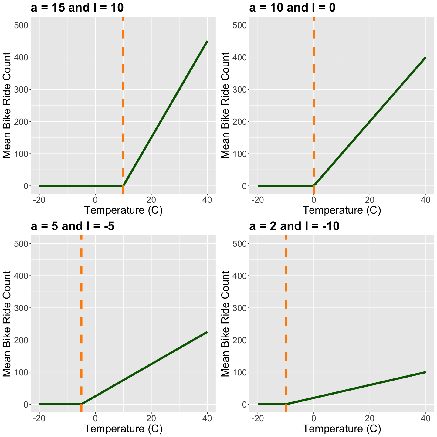
../_images/1f8c8791324d1cc3d50060840b70045d59d3757447989c0814ed67eba78d95fe.png

Exercise 13

Descriptively, what is the behaviour of our modelling function for $\lambda_w(t)$?

3.2. Modelling the Weather Parameters#

We know weather status is categorical, temperature is real, and the number of rides is a non-negative integer count. Moreover, let us assume weather status and temperature are fixed covariates (we are not trying to model them). The counts will be Poisson distributed.

Nonetheless, our previous modelling of the behaviour of $\lambda_{w_i}(t_i)$ yielded six different parameters we need to model! Thus, let us find some suitable distributions for:

$a_w$ with $w\in\{1,2,3\}$.
$l_w$ with $w\in\{1,2,3\}$.

Our previous plots with different values of $a_w$ and $l_w$ shed light on what class of distributions will be suitable in our model:

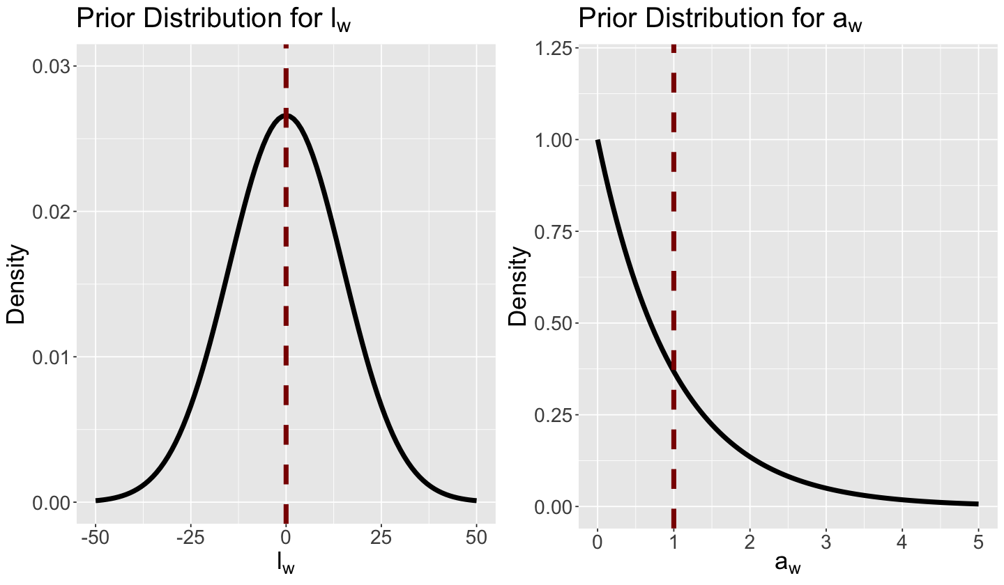
For the CONTINUOUS slopes $a_w$, we will assume they will only take on nonnegative values. A handy distribution for this case is the Gamma distribution
On the other hand, we will allow the CONTINUOUS elbows $l_w$ to take on any real value. Thus, the Normal distribution.

Gamma Distribution	Normal Distribution

Sources:

Gamma distribution. (2025, January 14). In Wikipedia. https://en.wikipedia.org/wiki/Gamma_distribution

Normal distribution. (2025, January 26). In Wikipedia. https://en.wikipedia.org/wiki/Normal_distribution

Therefore, our prior distributions for these weather parameters would be:

\[\begin{split}\begin{gather*} l_w \sim \mathcal{N}(\mu, \sigma^2) \quad \text{for} \quad w\in\{1,2,3\} \\ a_w \sim \mathrm{Gamma}(k, \theta) \quad \text{for} \quad w\in\{1,2,3\}. \end{gather*}\end{split}\]

Now, we have hyperparameters! They are $\mu$, $\sigma^2$, $k$ and $\theta$.

Moreover, we will make them reflect uncertainty:

\[\begin{split}\begin{gather*} \mu = 0 \\ \sigma^2 = 15^2 = 225 \\ k = 1 \\ \theta = 1. \end{gather*}\end{split}\]

The corresponding prior distributions for $l_w$ and $a_w$ are plotted below (the prior means are the vertical dashed red lines). Note we are giving considerable uncertainty to $l_w$ while allowing any real number. On the other hand, we restrict $a_w$ to nonnegative numbers while allocating larger probabilities to small values (i.e., we are not expecting large rates of change for the mean counts of bike rides).

plot_grid(prior_l_w, prior_a_w)

../_images/ac3197f63760d203e0b4a10ac52944ff15e91b5ef4c9588c34f101cd3f078b54.png

Finally, with a dataset containing $n$ observations (i.e., rows in bikeshare_data), for the $i$th observation $(i = 1, \dots, n)$ with temperature $t_i$:

\[\begin{split}\begin{align*} \text{likelihood:} \qquad R_i \mid a_{w_i}, l_{w_i} \mathop\sim^\text{ind} \text{Poisson}\left(\lambda_{w_i}(t_i)\right) \\ \text{where} \quad \lambda_{w_i}(t_i) = \log\{1+\exp[a_{w_i} (t_i - l_{w_i})]\} \quad \text{and} \quad w_i \in \{1, 2, 3\} \\ \text{priors:} \quad a_{w_i} \sim \mathrm{Gamma}(k = 1, \theta = 1) \\ \qquad l_{w_i} \sim \mathcal{N}(\mu = 0, \sigma^2 = 15^2). \end{align*}\end{split}\]

4. Overview of Markov Chain Monte Carlo#

In general, a Bayesian model will have $d$ parameters of interest for which we will need to obtain a joint posterior distribution:

\[\Theta = (\theta_1, \dots, \theta_d)^T.\]

Recall the Bayes’ rule:

\[\text{posterior} = \frac{\text{prior} \times \text{likelihood}}{\text{normalizing constant}} \propto \text{prior} \times \text{likelihood}.\]

Using $\Theta$ as our parameter vector of interest, let $f(\Theta)$ be the multivariate joint prior. Moreover with our observed data $\mathbf{y} = (y_1, \dots, y_n)^T$, let $\mathscr{l}(\Theta \mid \mathbf{y})$ be the corresponding multivariate likelihood function along with the multivariate normalizing constant $f(\mathbf{y})$.

Then, for the multivariate joint posterior $f(\Theta \mid \mathbf{y})$, the Bayes’ rule becomes:

\[f(\Theta \mid \mathbf{y}) = \frac{f(\Theta) \times \mathscr{l}(\Theta \mid \mathbf{y})}{f(\mathbf{y})} \propto f(\Theta) \times \mathscr{l}(\Theta \mid \mathbf{y}).\]

Why are we highlighting multivariate all the time? It is because we have $d$ parameters in vector $\Theta$.

Suppose we want to obtain an analytical form for $f(\mathbf{y})$, then this will be an integral to solve:

\[f(\mathbf{y}) = \int_{\theta_1} \int_{\theta_2} \cdots \int_{\theta_d} f(\Theta) \mathscr{l}(\Theta \mid \mathbf{y}) d\theta_d\ \cdots d\theta_1.\]

Solving this multivariate integral looks pretty challenging! Nonetheless, recall we do not need to obtain $f(\mathbf{y})$, but we still need to work around the math in

\[f(\Theta \mid \mathbf{y}) \propto f(\Theta) \times \mathscr{l}(\Theta \mid \mathbf{y}).\]

Important

Cases such as the Beta-Binomial and Gamma-Poisson are well behaved and approachable for parameters $\pi$ and $\lambda$, respectively. Therefore, we can obtain a closed solution for the corresponding posterior distribution.

But, what can we do when we have a whole set of parameters in vector $\Theta$? It will not be possible to find an exact form for $f(\Theta \mid \mathbf{y})$, but it is possible to approximate it via an algorithm!

Let us explore the MCMC algorithm by parts: Markov Chain and Monte Carlo.

4.1. Monte Carlo Algorithm#

We will start with the simple Monte Carlo algorithm. Suppose you have a closed analytical form for the posterior distribution $f(\Theta \mid \mathbf{y})$ (e.g., the Beta posterior in the Beta-Binomial model). You can build your independent Monte Carlo sample $\{ \Theta_1, \dots, \Theta_N \}$ of size $N$, from $f(\Theta \mid \mathbf{y})$ by selecting each element $\Theta_i$ ($i = 1, \dots, N$) in the following way:

Step 1. Draw $\Theta_i$ from $f(\Theta \mid \mathbf{y})$.
Step 2. Go there.

This is a random walk!

Caution

Drawing fully independent elements for our sample WILL NOT be possible in MCMC. Moreover, note that $n \neq N$.

4.2. Markov Chain#

Here comes the MCMC twist to the previous Monte Carlo approach: Markov Chain.

What is a Markov Chain? In terms of our Bayesian modelling for the posterior, it is a sequence $\{ \Theta_1, \dots, \Theta_N \}$ of size $N$ whose elements are NOT ENTIRELY INDEPENDENT (hence the word chain!).

What does NOT ENTIRELY INDEPENDENT implicate? It implicates the so-called Markov property:

The next sampled $\Theta_{i + 1}$ will depend on the current $\Theta_{i}$ but not on previous $\Theta_{i - 1}, \Theta_{i - 2}, \dots$

More formally, because of this property, the conditional probability function of $\Theta_{i + 1}$ can be depicted as:

\[f(\Theta_{i + 1} \mid \Theta_{i}, \mathbf{y}) = f(\Theta_{i + 1} \mid \Theta_1, \Theta_2, \dots \Theta_{i}, \mathbf{y}).\]

Again, there is no free lunch here! Each element in this chain can be drawn from another distribution and not specifically from our target posterior $f(\Theta \mid \mathbf{y})$:

\[f(\Theta_{i + 1} \mid \Theta_{i}, \mathbf{y}) \neq f(\Theta_{i + 1} \mid \mathbf{y}).\]

Thus, what is the point of this Markov Chain approach? The answer lies in the MCMC algorithm that approximates $f(\Theta \mid \mathbf{y})$ via our $N$ elements in the chain.

Important

There is more than one MCMC algorithm to do so, and the foundational one is the Metropolis-Hastings algorithm.

4.3. The Metropolis-Hastings Algorithm#

This is the algorithm that will allow us to obtain an approximation of the posterior distribution $f(\Theta \mid \mathbf{y})$ via our Markov Chain $\{ \Theta_1, \dots, \Theta_N \}$. Hence, with $\Theta_i$ in our current iteration $(i = 1, 2, \dots, N - 1)$, the next iteration $\Theta_{i + 1}$ will be selected through a two-step process.

Recall the Bayes’ rule:

\[f(\Theta \mid \mathbf{y}) \propto f(\Theta) \times \mathscr{l}(\Theta \mid \mathbf{y}).\]

Let the current $\Theta_i = \Theta$. Then, the algorithm’s two steps are:

Step 1. Randomly draw a new location $\Theta'$ from a proposed model with PDF $q(\Theta' \mid \Theta)$. This proposed model is what we call a jumping distribution and it could be a Uniform or Normal which are symmetric.

Important

Another choice of a jumping distribution could be asymmetric, such as the Log-normal. We can choose this jumping distribution class when there are constraints on our parameters of interest (e.g., they are nonnegative), or we want to sample large values from the chain (recall the Log-normal is a heavy-tailed distribution).

Step 2. Now, let us decide to go or not to go to the proposed $\Theta'$:

Important

Step 2 is divided in two parts:

a. Compute the acceptance probability for $\Theta'$:

\[\alpha = \min \bigg\{ 1, \frac{f(\Theta') \mathscr{l}(\Theta' \mid \mathbf{y})}{f(\Theta) \mathscr{l}(\Theta \mid \mathbf{y})} \times \frac{q(\Theta \mid \Theta')}{q(\Theta' \mid \Theta)} \bigg\}.\]

b. Obtain the next location $\Theta_{i + 1}$ as a Bernoulli trial (flipping an unfair coin!) taking on the two possible values:

\[\begin{split} \Theta_{i + 1} = \begin{cases} \Theta' \; \; \; \; \mbox{with probability } \alpha\\ \Theta \; \; \; \; \mbox{with probability } 1 -\alpha. \end{cases} \end{split}\]

4.4. The Metropolis Algorithm#

The previous Metropolis-Hastings algorithm can be simplified when the PDF of the jumping distribution is Uniform such that:

\[\begin{split}\begin{equation*} q(\Theta' \mid \Theta) = q(\Theta \mid \Theta') = \begin{cases} \frac{1}{2w} \; \; \; \; \mbox{when $\Theta$ and $\Theta'$ are within $w$ units of each other} \\ 0 \; \; \; \; \mbox{otherwise.} \end{cases} \end{equation*}\end{split}\]

This jumping distribution allocates the same probability of switching from $\Theta$ to $\Theta'$ compared to switching from $\Theta'$ to $\Theta$. Note that $w$ is the window parameter. Having said that, the definition of $\alpha$ will change to:

\[\alpha = \min \bigg\{ 1, \frac{f(\Theta') \mathscr{l}(\Theta' \mid \mathbf{y})}{f(\Theta) \mathscr{l}(\Theta \mid \mathbf{y})} \bigg\}.\]

4.5. Other MCMC Algorithms#

Metropolis-Hastings and its simplified Metropolis version are only a couple of MCMC tools. These two approaches target single parameters (e.g., a probability of success $\pi$ or a mean $\lambda$). However, when we want to deal with $d$ parameters, such as $\Theta = (\theta_1, \dots, \theta_d)^T$, there are more complex tools like Gibbs sampling (used in JAGS, Just Another Gibbs Sampler) or the No-U-Turn sampler (NUTS) which is a Hamiltonian Monte Carlo (HMC) algorithm (implemented in Stan).

4.6. Important Facts to Consider when `sampling()` via `rstan`#

The MCMC algorithm has a learning curve; thus, the Markov Chain initially starts sampling unreasonable numbers to approximate the posterior $f(\Theta \mid \mathbf{y})$. Therefore, we have a burn-in stage at the beginning of sampling() defined by the parameter warmup. This parameter will discard the first warmup iterations for the final simulation output.

Recall that consecutive elements in the chain are not independent. Hence, given the Markov property, we could skip draws between our definitive sampled values throughout the simulation to achieve a certain degree of sampling independence. This is defined by thin.

Important

We will obtain the following number of approximate posterior samples via sampling():

\[\texttt{Number of approximate posterior samples} = \frac{\texttt{iter} - \texttt{warmup}}{\texttt{thin}}.\]

5. Using `Stan` to Obtain our Posterior Distribution#

We already designed our Bayesian model. Now it is time to code it in Stan. Recall that with a dataset containing $n$ observations (i.e., rows in bikeshare_data which is our training set size), for the $i$th observation $(i = 1, \dots, n)$ with temperature $t_i$:

\[\begin{split}\begin{align*} \text{likelihood:} \qquad R_i \mid a_{w_i}, l_{w_i} \mathop\sim^\text{ind} \text{Poisson}\big(\lambda_{w_i}(t_i)\big) \\ \text{where} \quad \lambda_{w_i}(t_i) = \log\{1+\exp[a_{w_i} (t_i - l_{w_i})]\} \quad \text{and} \quad w_i \in \{1, 2, 3\} \\ \text{priors:} \quad a_{w_i} \sim \mathrm{Gamma}(k = 1, \theta = 1) \\ \qquad l_{w_i} \sim \mathcal{N}(\mu = 0, \sigma^2 = 15^2). \end{align*}\end{split}\]

5.1. Coding the Model#

Recall Stan has a block structure. Therefore, we will use the following blocks:

data: The inputs needed to run the Bayesian model.
parameters: The parameters to be sampled for our posterior analysis ($a_w$ and $l_w$ for $w \in \{1, 2, 3\}$). Their approximate posterior distributions will allow us to establish the extent to which temperature and mean bike ride count are related across different categories of weather (this is Bayesian inference!).
model: Our Bayesian model.

Caution

Stan needs to know every single detail of our data and generative model (object types, sizes, loops, etc.).

Unlike the R markdown, we do not have a Stan cell in Jupyter notebook/lab. Hence, we need to code our bikeshare_model as a string.

bikeshare_model <- "data {                          
int<lower=1> number_weather_cat;      // integer to indicate how many weather categories we have
int<lower=1> n;      // how many rows we have in bikeshare_data                               
vector[n] temp;      // column bikeshare_data$temp of real type
int<lower=1> weather[n];      // column bikeshare_data$weather as integer                      
int<lower=0> ride_count[n];      // column bikeshare_data$ride_count as integer                    
}
parameters {
vector<lower=0>[number_weather_cat] a;      // a vector of size number_weather_cat for a_w
vector[number_weather_cat] l;      // a real-type vector of size number_weather_cat for l_w
}
model {
for (j in 1:number_weather_cat){      // we have three PAIRS of priors, i.e., one PAIR per weather category
  a[j] ~ gamma(1, 1);
  l[j] ~ normal(0, 15);
}
for (i in 1:n){      // building our likelihood
  int w_index = weather[i];      // auxiliary variable for the ith weather category
  ride_count[i] ~ poisson(log(1 + exp(a[w_index] * (temp[i] - l[w_index]))));
}
}"

5.2. MCMC Simulation#

Next, we create a dictionary with all the data variables we need to pass into Stan as a list().

bikeshare_dictionary <- list(
  number_weather_cat = 3,
  n = nrow(bikeshare_data), 
  temp = bikeshare_data$temp,
  weather = as.integer(bikeshare_data$weather),
  ride_count = as.integer(bikeshare_data$ride_count)
)

We have not compiled bikeshare_model. Hence, we cannot use sampling() directly but stan() as in the cell below. Note the MCMC arguments are provided as in sampling():

chains: How many times we want to run the Bayesian simulation.
iter: The number of approximate posterior sampled sets of parameters we want (including burn-in).
warmup: The burn-in period.
thin: Number of samples to skip between each draw.
seed: Reproducibility seed.

posterior_bikeshare <- stan(
  model_code = bikeshare_model,
  data = bikeshare_dictionary,
  chains = 1,
  iter = 20000,
  warmup = 2000,
  thin = 40,
  seed = 553,
  verbose = TRUE,
  algorithm = "NUTS"
)

Show code cell output Hide code cell output

TRANSLATING MODEL '' FROM Stan CODE TO C++ CODE NOW.
OS: aarch64, darwin20; rstan: 2.32.6; Rcpp: 1.0.12; inline: 0.3.19 
 >> setting environment variables: 
PKG_LIBS =  '/Library/Frameworks/R.framework/Versions/4.4-arm64/Resources/library/rstan/lib//libStanServices.a' -L'/Library/Frameworks/R.framework/Versions/4.4-arm64/Resources/library/StanHeaders/lib/' -lStanHeaders -L'/Library/Frameworks/R.framework/Versions/4.4-arm64/Resources/library/RcppParallel/lib/' -ltbb -L/Library/Frameworks/R.framework/Versions/4.4-arm64/Resources/library/RcppParallel/lib -ltbb -ltbbmalloc
PKG_CPPFLAGS =   -I"/Library/Frameworks/R.framework/Versions/4.4-arm64/Resources/library/Rcpp/include/"  -I"/Library/Frameworks/R.framework/Versions/4.4-arm64/Resources/library/RcppEigen/include/"  -I"/Library/Frameworks/R.framework/Versions/4.4-arm64/Resources/library/RcppEigen/include/unsupported"  -I"/Library/Frameworks/R.framework/Versions/4.4-arm64/Resources/library/BH/include" -I"/Library/Frameworks/R.framework/Versions/4.4-arm64/Resources/library/StanHeaders/include/src/"  -I"/Library/Frameworks/R.framework/Versions/4.4-arm64/Resources/library/StanHeaders/include/"  -I"/Library/Frameworks/R.framework/Versions/4.4-arm64/Resources/library/RcppParallel/include/"  -I"/Library/Frameworks/R.framework/Versions/4.4-arm64/Resources/library/rstan/include" -DEIGEN_NO_DEBUG  -DBOOST_DISABLE_ASSERTS  -DBOOST_PENDING_INTEGER_LOG2_HPP  -DSTAN_THREADS  -DUSE_STANC3 -DSTRICT_R_HEADERS  -DBOOST_PHOENIX_NO_VARIADIC_EXPRESSION  -D_HAS_AUTO_PTR_ETC=0  -include '/Library/Frameworks/R.framework/Versions/4.4-arm64/Resources/library/StanHeaders/include/stan/math/prim/fun/Eigen.hpp'  -D_REENTRANT -DRCPP_PARALLEL_USE_TBB=1 
 >> Program source :

: 
: // includes from the plugin
: // [[Rcpp::plugins(cpp14)]]
: 
: 
: // user includes
: #include <Rcpp.h>
: using namespace Rcpp;
: #ifndef MODELS_HPP
: #define MODELS_HPP
: #define STAN__SERVICES__COMMAND_HPP
: #include <rstan/rstaninc.hpp>
: #ifndef USE_STANC3
: #define USE_STANC3
: #endif
: // Code generated by stanc v2.32.2
: #include <stan/model/model_header.hpp>
: namespace model18558745e4a24__namespace {
: using stan::model::model_base_crtp;
: using namespace stan::math;
: stan::math::profile_map profiles__;
: static constexpr std::array<const char*, 21> locations_array__ =
:   {" (found before start of program)",
:   " (in 'anon_model', line 9, column 0 to column 38)",
:   " (in 'anon_model', line 10, column 0 to column 29)",
:   " (in 'anon_model', line 14, column 2 to column 21)",
:   " (in 'anon_model', line 15, column 2 to column 23)",
:   " (in 'anon_model', line 13, column 31 to line 16, column 1)",
:   " (in 'anon_model', line 13, column 0 to line 16, column 1)",
:   " (in 'anon_model', line 18, column 2 to column 27)",
:   " (in 'anon_model', line 19, column 2 to column 77)",
:   " (in 'anon_model', line 17, column 14 to line 20, column 1)",
:   " (in 'anon_model', line 17, column 0 to line 20, column 1)",
:   " (in 'anon_model', line 2, column 0 to column 32)",
:   " (in 'anon_model', line 3, column 0 to column 15)",
:   " (in 'anon_model', line 4, column 7 to column 8)",
:   " (in 'anon_model', line 4, column 0 to column 15)",
:   " (in 'anon_model', line 5, column 21 to column 22)",
:   " (in 'anon_model', line 5, column 0 to column 24)",
:   " (in 'anon_model', line 6, column 24 to column 25)",
:   " (in 'anon_model', line 6, column 0 to column 27)",
:   " (in 'anon_model', line 9, column 16 to column 34)",
:   " (in 'anon_model', line 10, column 7 to column 25)"};
: class model18558745e4a24_ final : public model_base_crtp<model18558745e4a24_> {
: private:
:   int number_weather_cat;
:   int n;
:   Eigen::Matrix<double,-1,1> temp_data__;
:   std::vector<int> weather;
:   std::vector<int> ride_count;
:   Eigen::Map<Eigen::Matrix<double,-1,1>> temp{nullptr, 0};
: public:
:   ~model18558745e4a24_() {}
:   model18558745e4a24_(stan::io::var_context& context__, unsigned int
:                       random_seed__ = 0, std::ostream* pstream__ = nullptr)
:       : model_base_crtp(0) {
:     int current_statement__ = 0;
:     using local_scalar_t__ = double;
:     boost::ecuyer1988 base_rng__ =
:       stan::services::util::create_rng(random_seed__, 0);
:     // suppress unused var warning
:     (void) base_rng__;
:     static constexpr const char* function__ =
:       "model18558745e4a24__namespace::model18558745e4a24_";
:     // suppress unused var warning
:     (void) function__;
:     local_scalar_t__ DUMMY_VAR__(std::numeric_limits<double>::quiet_NaN());
:     // suppress unused var warning
:     (void) DUMMY_VAR__;
:     try {
:       int pos__ = std::numeric_limits<int>::min();
:       pos__ = 1;
:       current_statement__ = 11;
:       context__.validate_dims("data initialization", "number_weather_cat",
:         "int", std::vector<size_t>{});
:       number_weather_cat = std::numeric_limits<int>::min();
:       current_statement__ = 11;
:       number_weather_cat = context__.vals_i("number_weather_cat")[(1 - 1)];
:       current_statement__ = 11;
:       stan::math::check_greater_or_equal(function__, "number_weather_cat",
:         number_weather_cat, 1);
:       current_statement__ = 12;
:       context__.validate_dims("data initialization", "n", "int",
:         std::vector<size_t>{});
:       n = std::numeric_limits<int>::min();
:       current_statement__ = 12;
:       n = context__.vals_i("n")[(1 - 1)];
:       current_statement__ = 12;
:       stan::math::check_greater_or_equal(function__, "n", n, 1);
:       current_statement__ = 13;
:       stan::math::validate_non_negative_index("temp", "n", n);
:       current_statement__ = 14;
:       context__.validate_dims("data initialization", "temp", "double",
:         std::vector<size_t>{static_cast<size_t>(n)});
:       temp_data__ = Eigen::Matrix<double,-1,1>::Constant(n,
:                       std::numeric_limits<double>::quiet_NaN());
:       new (&temp) Eigen::Map<Eigen::Matrix<double,-1,1>>(temp_data__.data(),
:         n);
:       {
:         std::vector<local_scalar_t__> temp_flat__;
:         current_statement__ = 14;
:         temp_flat__ = context__.vals_r("temp");
:         current_statement__ = 14;
:         pos__ = 1;
:         current_statement__ = 14;
:         for (int sym1__ = 1; sym1__ <= n; ++sym1__) {
:           current_statement__ = 14;
:           stan::model::assign(temp, temp_flat__[(pos__ - 1)],
:             "assigning variable temp", stan::model::index_uni(sym1__));
:           current_statement__ = 14;
:           pos__ = (pos__ + 1);
:         }
:       }
:       current_statement__ = 15;
:       stan::math::validate_non_negative_index("weather", "n", n);
:       current_statement__ = 16;
:       context__.validate_dims("data initialization", "weather", "int",
:         std::vector<size_t>{static_cast<size_t>(n)});
:       weather = std::vector<int>(n, std::numeric_limits<int>::min());
:       current_statement__ = 16;
:       weather = context__.vals_i("weather");
:       current_statement__ = 16;
:       stan::math::check_greater_or_equal(function__, "weather", weather, 1);
:       current_statement__ = 17;
:       stan::math::validate_non_negative_index("ride_count", "n", n);
:       current_statement__ = 18;
:       context__.validate_dims("data initialization", "ride_count", "int",
:         std::vector<size_t>{static_cast<size_t>(n)});
:       ride_count = std::vector<int>(n, std::numeric_limits<int>::min());
:       current_statement__ = 18;
:       ride_count = context__.vals_i("ride_count");
:       current_statement__ = 18;
:       stan::math::check_greater_or_equal(function__, "ride_count",
:         ride_count, 0);
:       current_statement__ = 19;
:       stan::math::validate_non_negative_index("a", "number_weather_cat",
:         number_weather_cat);
:       current_statement__ = 20;
:       stan::math::validate_non_negative_index("l", "number_weather_cat",
:         number_weather_cat);
:     } catch (const std::exception& e) {
:       stan::lang::rethrow_located(e, locations_array__[current_statement__]);
:     }
:     num_params_r__ = number_weather_cat + number_weather_cat;
:   }
:   inline std::string model_name() const final {
:     return "model18558745e4a24_";
:   }
:   inline std::vector<std::string> model_compile_info() const noexcept {
:     return std::vector<std::string>{"stanc_version = stanc3 v2.32.2",
:              "stancflags = --"};
:   }
:   template <bool propto__, bool jacobian__, typename VecR, typename VecI,
:             stan::require_vector_like_t<VecR>* = nullptr,
:             stan::require_vector_like_vt<std::is_integral, VecI>* = nullptr>
:   inline stan::scalar_type_t<VecR>
:   log_prob_impl(VecR& params_r__, VecI& params_i__, std::ostream*
:                 pstream__ = nullptr) const {
:     using T__ = stan::scalar_type_t<VecR>;
:     using local_scalar_t__ = T__;
:     T__ lp__(0.0);
:     stan::math::accumulator<T__> lp_accum__;
:     stan::io::deserializer<local_scalar_t__> in__(params_r__, params_i__);
:     int current_statement__ = 0;
:     local_scalar_t__ DUMMY_VAR__(std::numeric_limits<double>::quiet_NaN());
:     // suppress unused var warning
:     (void) DUMMY_VAR__;
:     static constexpr const char* function__ =
:       "model18558745e4a24__namespace::log_prob";
:     // suppress unused var warning
:     (void) function__;
:     try {
:       Eigen::Matrix<local_scalar_t__,-1,1> a =
:         Eigen::Matrix<local_scalar_t__,-1,1>::Constant(number_weather_cat,
:           DUMMY_VAR__);
:       current_statement__ = 1;
:       a = in__.template read_constrain_lb<
:             Eigen::Matrix<local_scalar_t__,-1,1>, jacobian__>(0, lp__,
:             number_weather_cat);
:       Eigen::Matrix<local_scalar_t__,-1,1> l =
:         Eigen::Matrix<local_scalar_t__,-1,1>::Constant(number_weather_cat,
:           DUMMY_VAR__);
:       current_statement__ = 2;
:       l = in__.template read<
:             Eigen::Matrix<local_scalar_t__,-1,1>>(number_weather_cat);
:       {
:         current_statement__ = 6;
:         for (int j = 1; j <= number_weather_cat; ++j) {
:           current_statement__ = 3;
:           lp_accum__.add(stan::math::gamma_lpdf<propto__>(
:                            stan::model::rvalue(a, "a",
:                              stan::model::index_uni(j)), 1, 1));
:           current_statement__ = 4;
:           lp_accum__.add(stan::math::normal_lpdf<propto__>(
:                            stan::model::rvalue(l, "l",
:                              stan::model::index_uni(j)), 0, 15));
:         }
:         current_statement__ = 10;
:         for (int i = 1; i <= n; ++i) {
:           int w_index = std::numeric_limits<int>::min();
:           current_statement__ = 7;
:           w_index = stan::model::rvalue(weather, "weather",
:                       stan::model::index_uni(i));
:           current_statement__ = 8;
:           lp_accum__.add(stan::math::poisson_lpmf<propto__>(
:                            stan::model::rvalue(ride_count, "ride_count",
:                              stan::model::index_uni(i)),
:                            stan::math::log((1 +
:                              stan::math::exp(
:                                (stan::model::rvalue(a, "a",
:                                   stan::model::index_uni(w_index)) *
:                                (stan::model::rvalue(temp, "temp",
:                                   stan::model::index_uni(i)) -
:                                stan::model::rvalue(l, "l",
:                                  stan::model::index_uni(w_index)))))))));
:         }
:       }
:     } catch (const std::exception& e) {
:       stan::lang::rethrow_located(e, locations_array__[current_statement__]);
:     }
:     lp_accum__.add(lp__);
:     return lp_accum__.sum();
:   }
:   template <typename RNG, typename VecR, typename VecI, typename VecVar,
:             stan::require_vector_like_vt<std::is_floating_point,
:             VecR>* = nullptr, stan::require_vector_like_vt<std::is_integral,
:             VecI>* = nullptr, stan::require_vector_vt<std::is_floating_point,
:             VecVar>* = nullptr>
:   inline void
:   write_array_impl(RNG& base_rng__, VecR& params_r__, VecI& params_i__,
:                    VecVar& vars__, const bool
:                    emit_transformed_parameters__ = true, const bool
:                    emit_generated_quantities__ = true, std::ostream*
:                    pstream__ = nullptr) const {
:     using local_scalar_t__ = double;
:     stan::io::deserializer<local_scalar_t__> in__(params_r__, params_i__);
:     stan::io::serializer<local_scalar_t__> out__(vars__);
:     static constexpr bool propto__ = true;
:     // suppress unused var warning
:     (void) propto__;
:     double lp__ = 0.0;
:     // suppress unused var warning
:     (void) lp__;
:     int current_statement__ = 0;
:     stan::math::accumulator<double> lp_accum__;
:     local_scalar_t__ DUMMY_VAR__(std::numeric_limits<double>::quiet_NaN());
:     // suppress unused var warning
:     (void) DUMMY_VAR__;
:     constexpr bool jacobian__ = false;
:     static constexpr const char* function__ =
:       "model18558745e4a24__namespace::write_array";
:     // suppress unused var warning
:     (void) function__;
:     try {
:       Eigen::Matrix<double,-1,1> a =
:         Eigen::Matrix<double,-1,1>::Constant(number_weather_cat,
:           std::numeric_limits<double>::quiet_NaN());
:       current_statement__ = 1;
:       a = in__.template read_constrain_lb<
:             Eigen::Matrix<local_scalar_t__,-1,1>, jacobian__>(0, lp__,
:             number_weather_cat);
:       Eigen::Matrix<double,-1,1> l =
:         Eigen::Matrix<double,-1,1>::Constant(number_weather_cat,
:           std::numeric_limits<double>::quiet_NaN());
:       current_statement__ = 2;
:       l = in__.template read<
:             Eigen::Matrix<local_scalar_t__,-1,1>>(number_weather_cat);
:       out__.write(a);
:       out__.write(l);
:       if (stan::math::logical_negation(
:             (stan::math::primitive_value(emit_transformed_parameters__) ||
:             stan::math::primitive_value(emit_generated_quantities__)))) {
:         return ;
:       }
:       if (stan::math::logical_negation(emit_generated_quantities__)) {
:         return ;
:       }
:     } catch (const std::exception& e) {
:       stan::lang::rethrow_located(e, locations_array__[current_statement__]);
:     }
:   }
:   template <typename VecVar, typename VecI,
:             stan::require_vector_t<VecVar>* = nullptr,
:             stan::require_vector_like_vt<std::is_integral, VecI>* = nullptr>
:   inline void
:   unconstrain_array_impl(const VecVar& params_r__, const VecI& params_i__,
:                          VecVar& vars__, std::ostream* pstream__ = nullptr) const {
:     using local_scalar_t__ = double;
:     stan::io::deserializer<local_scalar_t__> in__(params_r__, params_i__);
:     stan::io::serializer<local_scalar_t__> out__(vars__);
:     int current_statement__ = 0;
:     local_scalar_t__ DUMMY_VAR__(std::numeric_limits<double>::quiet_NaN());
:     // suppress unused var warning
:     (void) DUMMY_VAR__;
:     try {
:       int pos__ = std::numeric_limits<int>::min();
:       pos__ = 1;
:       Eigen::Matrix<local_scalar_t__,-1,1> a =
:         Eigen::Matrix<local_scalar_t__,-1,1>::Constant(number_weather_cat,
:           DUMMY_VAR__);
:       current_statement__ = 1;
:       stan::model::assign(a,
:         in__.read<Eigen::Matrix<local_scalar_t__,-1,1>>(number_weather_cat),
:         "assigning variable a");
:       out__.write_free_lb(0, a);
:       Eigen::Matrix<local_scalar_t__,-1,1> l =
:         Eigen::Matrix<local_scalar_t__,-1,1>::Constant(number_weather_cat,
:           DUMMY_VAR__);
:       current_statement__ = 2;
:       stan::model::assign(l,
:         in__.read<Eigen::Matrix<local_scalar_t__,-1,1>>(number_weather_cat),
:         "assigning variable l");
:       out__.write(l);
:     } catch (const std::exception& e) {
:       stan::lang::rethrow_located(e, locations_array__[current_statement__]);
:     }
:   }
:   template <typename VecVar, stan::require_vector_t<VecVar>* = nullptr>
:   inline void
:   transform_inits_impl(const stan::io::var_context& context__, VecVar&
:                        vars__, std::ostream* pstream__ = nullptr) const {
:     using local_scalar_t__ = double;
:     stan::io::serializer<local_scalar_t__> out__(vars__);
:     int current_statement__ = 0;
:     local_scalar_t__ DUMMY_VAR__(std::numeric_limits<double>::quiet_NaN());
:     // suppress unused var warning
:     (void) DUMMY_VAR__;
:     try {
:       current_statement__ = 1;
:       context__.validate_dims("parameter initialization", "a", "double",
:         std::vector<size_t>{static_cast<size_t>(number_weather_cat)});
:       current_statement__ = 2;
:       context__.validate_dims("parameter initialization", "l", "double",
:         std::vector<size_t>{static_cast<size_t>(number_weather_cat)});
:       int pos__ = std::numeric_limits<int>::min();
:       pos__ = 1;
:       Eigen::Matrix<local_scalar_t__,-1,1> a =
:         Eigen::Matrix<local_scalar_t__,-1,1>::Constant(number_weather_cat,
:           DUMMY_VAR__);
:       {
:         std::vector<local_scalar_t__> a_flat__;
:         current_statement__ = 1;
:         a_flat__ = context__.vals_r("a");
:         current_statement__ = 1;
:         pos__ = 1;
:         current_statement__ = 1;
:         for (int sym1__ = 1; sym1__ <= number_weather_cat; ++sym1__) {
:           current_statement__ = 1;
:           stan::model::assign(a, a_flat__[(pos__ - 1)],
:             "assigning variable a", stan::model::index_uni(sym1__));
:           current_statement__ = 1;
:           pos__ = (pos__ + 1);
:         }
:       }
:       out__.write_free_lb(0, a);
:       Eigen::Matrix<local_scalar_t__,-1,1> l =
:         Eigen::Matrix<local_scalar_t__,-1,1>::Constant(number_weather_cat,
:           DUMMY_VAR__);
:       {
:         std::vector<local_scalar_t__> l_flat__;
:         current_statement__ = 2;
:         l_flat__ = context__.vals_r("l");
:         current_statement__ = 2;
:         pos__ = 1;
:         current_statement__ = 2;
:         for (int sym1__ = 1; sym1__ <= number_weather_cat; ++sym1__) {
:           current_statement__ = 2;
:           stan::model::assign(l, l_flat__[(pos__ - 1)],
:             "assigning variable l", stan::model::index_uni(sym1__));
:           current_statement__ = 2;
:           pos__ = (pos__ + 1);
:         }
:       }
:       out__.write(l);
:     } catch (const std::exception& e) {
:       stan::lang::rethrow_located(e, locations_array__[current_statement__]);
:     }
:   }
:   inline void
:   get_param_names(std::vector<std::string>& names__, const bool
:                   emit_transformed_parameters__ = true, const bool
:                   emit_generated_quantities__ = true) const {
:     names__ = std::vector<std::string>{"a", "l"};
:     if (emit_transformed_parameters__) {}
:     if (emit_generated_quantities__) {}
:   }
:   inline void
:   get_dims(std::vector<std::vector<size_t>>& dimss__, const bool
:            emit_transformed_parameters__ = true, const bool
:            emit_generated_quantities__ = true) const {
:     dimss__ = std::vector<std::vector<size_t>>{std::vector<size_t>{static_cast<
:                                                                     size_t>(
:                                                                     number_weather_cat)},
:                 std::vector<size_t>{static_cast<size_t>(number_weather_cat)}};
:     if (emit_transformed_parameters__) {}
:     if (emit_generated_quantities__) {}
:   }
:   inline void
:   constrained_param_names(std::vector<std::string>& param_names__, bool
:                           emit_transformed_parameters__ = true, bool
:                           emit_generated_quantities__ = true) const final {
:     for (int sym1__ = 1; sym1__ <= number_weather_cat; ++sym1__) {
:       param_names__.emplace_back(std::string() + "a" + '.' +
:         std::to_string(sym1__));
:     }
:     for (int sym1__ = 1; sym1__ <= number_weather_cat; ++sym1__) {
:       param_names__.emplace_back(std::string() + "l" + '.' +
:         std::to_string(sym1__));
:     }
:     if (emit_transformed_parameters__) {}
:     if (emit_generated_quantities__) {}
:   }
:   inline void
:   unconstrained_param_names(std::vector<std::string>& param_names__, bool
:                             emit_transformed_parameters__ = true, bool
:                             emit_generated_quantities__ = true) const final {
:     for (int sym1__ = 1; sym1__ <= number_weather_cat; ++sym1__) {
:       param_names__.emplace_back(std::string() + "a" + '.' +
:         std::to_string(sym1__));
:     }
:     for (int sym1__ = 1; sym1__ <= number_weather_cat; ++sym1__) {
:       param_names__.emplace_back(std::string() + "l" + '.' +
:         std::to_string(sym1__));
:     }
:     if (emit_transformed_parameters__) {}
:     if (emit_generated_quantities__) {}
:   }
:   inline std::string get_constrained_sizedtypes() const {
:     return std::string("[{\"name\":\"a\",\"type\":{\"name\":\"vector\",\"length\":" + std::to_string(number_weather_cat) + "},\"block\":\"parameters\"},{\"name\":\"l\",\"type\":{\"name\":\"vector\",\"length\":" + std::to_string(number_weather_cat) + "},\"block\":\"parameters\"}]");
:   }
:   inline std::string get_unconstrained_sizedtypes() const {
:     return std::string("[{\"name\":\"a\",\"type\":{\"name\":\"vector\",\"length\":" + std::to_string(number_weather_cat) + "},\"block\":\"parameters\"},{\"name\":\"l\",\"type\":{\"name\":\"vector\",\"length\":" + std::to_string(number_weather_cat) + "},\"block\":\"parameters\"}]");
:   }
:   // Begin method overload boilerplate
:   template <typename RNG> inline void
:   write_array(RNG& base_rng, Eigen::Matrix<double,-1,1>& params_r,
:               Eigen::Matrix<double,-1,1>& vars, const bool
:               emit_transformed_parameters = true, const bool
:               emit_generated_quantities = true, std::ostream*
:               pstream = nullptr) const {
:     const size_t num_params__ = (number_weather_cat + number_weather_cat);
:     const size_t num_transformed = emit_transformed_parameters * (0);
:     const size_t num_gen_quantities = emit_generated_quantities * (0);
:     const size_t num_to_write = num_params__ + num_transformed +
:       num_gen_quantities;
:     std::vector<int> params_i;
:     vars = Eigen::Matrix<double,-1,1>::Constant(num_to_write,
:              std::numeric_limits<double>::quiet_NaN());
:     write_array_impl(base_rng, params_r, params_i, vars,
:       emit_transformed_parameters, emit_generated_quantities, pstream);
:   }
:   template <typename RNG> inline void
:   write_array(RNG& base_rng, std::vector<double>& params_r, std::vector<int>&
:               params_i, std::vector<double>& vars, bool
:               emit_transformed_parameters = true, bool
:               emit_generated_quantities = true, std::ostream*
:               pstream = nullptr) const {
:     const size_t num_params__ = (number_weather_cat + number_weather_cat);
:     const size_t num_transformed = emit_transformed_parameters * (0);
:     const size_t num_gen_quantities = emit_generated_quantities * (0);
:     const size_t num_to_write = num_params__ + num_transformed +
:       num_gen_quantities;
:     vars = std::vector<double>(num_to_write,
:              std::numeric_limits<double>::quiet_NaN());
:     write_array_impl(base_rng, params_r, params_i, vars,
:       emit_transformed_parameters, emit_generated_quantities, pstream);
:   }
:   template <bool propto__, bool jacobian__, typename T_> inline T_
:   log_prob(Eigen::Matrix<T_,-1,1>& params_r, std::ostream* pstream = nullptr) const {
:     Eigen::Matrix<int,-1,1> params_i;
:     return log_prob_impl<propto__, jacobian__>(params_r, params_i, pstream);
:   }
:   template <bool propto__, bool jacobian__, typename T_> inline T_
:   log_prob(std::vector<T_>& params_r, std::vector<int>& params_i,
:            std::ostream* pstream = nullptr) const {
:     return log_prob_impl<propto__, jacobian__>(params_r, params_i, pstream);
:   }
:   inline void
:   transform_inits(const stan::io::var_context& context,
:                   Eigen::Matrix<double,-1,1>& params_r, std::ostream*
:                   pstream = nullptr) const final {
:     std::vector<double> params_r_vec(params_r.size());
:     std::vector<int> params_i;
:     transform_inits(context, params_i, params_r_vec, pstream);
:     params_r = Eigen::Map<Eigen::Matrix<double,-1,1>>(params_r_vec.data(),
:                  params_r_vec.size());
:   }
:   inline void
:   transform_inits(const stan::io::var_context& context, std::vector<int>&
:                   params_i, std::vector<double>& vars, std::ostream*
:                   pstream__ = nullptr) const {
:     vars.resize(num_params_r__);
:     transform_inits_impl(context, vars, pstream__);
:   }
:   inline void
:   unconstrain_array(const std::vector<double>& params_constrained,
:                     std::vector<double>& params_unconstrained, std::ostream*
:                     pstream = nullptr) const {
:     const std::vector<int> params_i;
:     params_unconstrained = std::vector<double>(num_params_r__,
:                              std::numeric_limits<double>::quiet_NaN());
:     unconstrain_array_impl(params_constrained, params_i,
:       params_unconstrained, pstream);
:   }
:   inline void
:   unconstrain_array(const Eigen::Matrix<double,-1,1>& params_constrained,
:                     Eigen::Matrix<double,-1,1>& params_unconstrained,
:                     std::ostream* pstream = nullptr) const {
:     const std::vector<int> params_i;
:     params_unconstrained = Eigen::Matrix<double,-1,1>::Constant(num_params_r__,
:                              std::numeric_limits<double>::quiet_NaN());
:     unconstrain_array_impl(params_constrained, params_i,
:       params_unconstrained, pstream);
:   }
: };
: }
: using stan_model = model18558745e4a24__namespace::model18558745e4a24_;
: #ifndef USING_R
: // Boilerplate
: stan::model::model_base&
: new_model(stan::io::var_context& data_context, unsigned int seed,
:           std::ostream* msg_stream) {
:   stan_model* m = new stan_model(data_context, seed, msg_stream);
:   return *m;
: }
: stan::math::profile_map& get_stan_profile_data() {
:   return model18558745e4a24__namespace::profiles__;
: }
: #endif
: #endif
: 
: RCPP_MODULE(stan_fit4model18558745e4a24__mod) {
:   class_<rstan::stan_fit<stan_model, boost::random::ecuyer1988> >(
:       "stan_fit4model18558745e4a24_")
: 
:       .constructor<SEXP, SEXP, SEXP>()
: 
:       .method(
:           "call_sampler",
:           &rstan::stan_fit<stan_model, boost::random::ecuyer1988>::call_sampler)
:       .method(
:           "param_names",
:           &rstan::stan_fit<stan_model, boost::random::ecuyer1988>::param_names)
:       .method("param_names_oi",
:               &rstan::stan_fit<stan_model,
:                                boost::random::ecuyer1988>::param_names_oi)
:       .method("param_fnames_oi",
:               &rstan::stan_fit<stan_model,
:                                boost::random::ecuyer1988>::param_fnames_oi)
:       .method(
:           "param_dims",
:           &rstan::stan_fit<stan_model, boost::random::ecuyer1988>::param_dims)
:       .method("param_dims_oi",
:               &rstan::stan_fit<stan_model,
:                                boost::random::ecuyer1988>::param_dims_oi)
:       .method("update_param_oi",
:               &rstan::stan_fit<stan_model,
:                                boost::random::ecuyer1988>::update_param_oi)
:       .method("param_oi_tidx",
:               &rstan::stan_fit<stan_model,
:                                boost::random::ecuyer1988>::param_oi_tidx)
:       .method("grad_log_prob",
:               &rstan::stan_fit<stan_model,
:                                boost::random::ecuyer1988>::grad_log_prob)
:       .method("log_prob",
:               &rstan::stan_fit<stan_model, boost::random::ecuyer1988>::log_prob)
:       .method("unconstrain_pars",
:               &rstan::stan_fit<stan_model,
:                                boost::random::ecuyer1988>::unconstrain_pars)
:       .method("constrain_pars",
:               &rstan::stan_fit<stan_model,
:                                boost::random::ecuyer1988>::constrain_pars)
:       .method(
:           "num_pars_unconstrained",
:           &rstan::stan_fit<stan_model,
:                            boost::random::ecuyer1988>::num_pars_unconstrained)
:       .method(
:           "unconstrained_param_names",
:           &rstan::stan_fit<
:               stan_model, boost::random::ecuyer1988>::unconstrained_param_names)
:       .method(
:           "constrained_param_names",
:           &rstan::stan_fit<stan_model,
:                            boost::random::ecuyer1988>::constrained_param_names)
:       .method("standalone_gqs",
:               &rstan::stan_fit<stan_model,
:                                boost::random::ecuyer1988>::standalone_gqs);
: }
: 
: 
: // declarations
: extern "C" {
: SEXP file185584cdbff65( ) ;
: }
: 
: // definition
: SEXP file185584cdbff65() {
:  return Rcpp::wrap("anon_model");
: }

CHECKING DATA AND PREPROCESSING FOR MODEL 'anon_model' NOW.

COMPILING MODEL 'anon_model' NOW.

STARTING SAMPLER FOR MODEL 'anon_model' NOW.

SAMPLING FOR MODEL 'anon_model' NOW (CHAIN 1).
Chain 1: 
Chain 1: Gradient evaluation took 0.001781 seconds
Chain 1: 1000 transitions using 10 leapfrog steps per transition would take 17.81 seconds.
Chain 1: Adjust your expectations accordingly!
Chain 1: 
Chain 1: 
Chain 1: Iteration:     1 / 20000 [  0%]  (Warmup)
Chain 1: Iteration:  2000 / 20000 [ 10%]  (Warmup)
Chain 1: Iteration:  2001 / 20000 [ 10%]  (Sampling)
Chain 1: Iteration:  4000 / 20000 [ 20%]  (Sampling)
Chain 1: Iteration:  6000 / 20000 [ 30%]  (Sampling)
Chain 1: Iteration:  8000 / 20000 [ 40%]  (Sampling)
Chain 1: Iteration: 10000 / 20000 [ 50%]  (Sampling)
Chain 1: Iteration: 12000 / 20000 [ 60%]  (Sampling)
Chain 1: Iteration: 14000 / 20000 [ 70%]  (Sampling)
Chain 1: Iteration: 16000 / 20000 [ 80%]  (Sampling)
Chain 1: Iteration: 18000 / 20000 [ 90%]  (Sampling)
Chain 1: Iteration: 20000 / 20000 [100%]  (Sampling)
Chain 1: 
Chain 1:  Elapsed Time: 63.03 seconds (Warm-up)
Chain 1:                507.332 seconds (Sampling)
Chain 1:                570.362 seconds (Total)
Chain 1: 

5.3. Obtaining, Visualizing, and Interpreting the Posterior Results#

posterior_bikeshare is our one-stop-shop!

We obtained a total of

\[\frac{\texttt{iter} - \texttt{warmup}}{\texttt{thin}} = \frac{20000 - 2000}{40} = 450\]

approximate posterior samples to be summarized in our inferential conclusions.

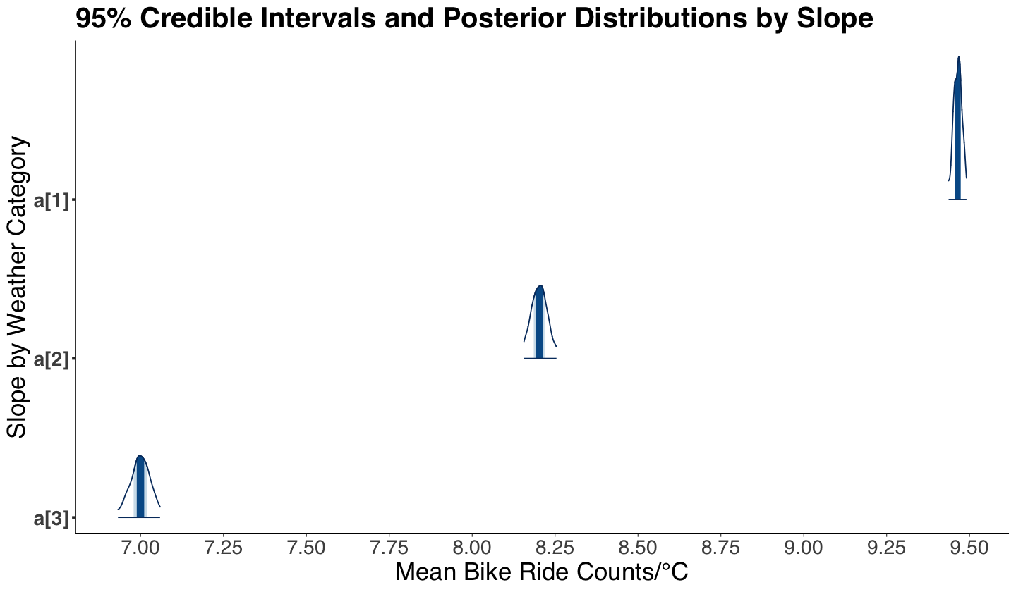
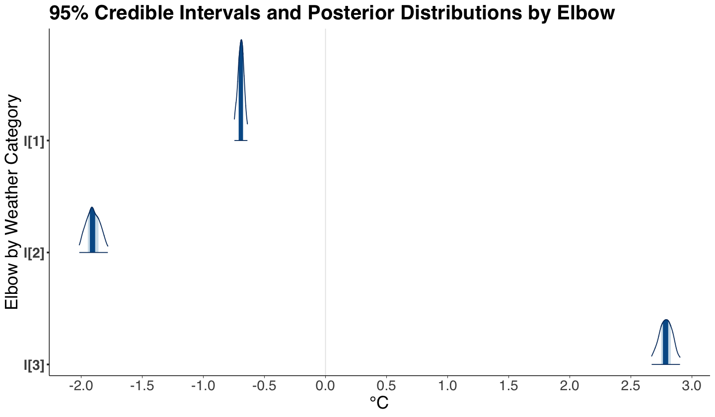
You can obtain the summary() statistics for the object posterior_bikeshare. These statistics are drawn from the approximate joint posterior distribution of the parameters of interest: $a_1$, $a_2$, $a_3$, $l_1$, $l_2$, and $l_3$. Lower and upper bounds for the 95% credible intervals are shown in columns 2.5% and 97.5%.

Metrics se_mean (Monte Carlo standard error), n_eff (effective sample size), and Rhat are model diagnostics (to be covered later on at the end of this course).

Attention

lp__ refers to the logarithm of the posterior joint density up to a constant that does not depend on the parameters of interest (we will not use it in this course).

You can find a useful optional resource if you are more interested in knowing how Stan performs its computation.

round(summary(posterior_bikeshare)$summary, 2)[-7, ]

A matrix: 6 × 10 of type dbl
	mean	sd	2.5%	25%	50%	75%	97.5%	n_eff	Rhat
a[1]	9.46	0.01	9.44	9.46	9.47	9.47	9.49	423.09	1
a[2]	8.20	0.03	8.16	8.19	8.20	8.22	8.25	427.82	1
a[3]	7.00	0.03	6.93	6.98	7.00	7.02	7.06	418.97	1
l[1]	-0.69	0.03	-0.75	-0.71	-0.69	-0.68	-0.64	454.05	1
l[2]	-1.90	0.06	-2.02	-1.95	-1.91	-1.86	-1.78	480.15	1
l[3]	2.78	0.06	2.67	2.75	2.78	2.83	2.90	398.77	1

Before plotting our posterior results, let us recheck the inferential inquiries:

How are temperature and weather associated with the mean number of trips?

Specifically, does the mean number of trips vary by the type of weather along with temperature?

How can we quantify this variation?

Now, we can also plot the six 95% credible intervals and posterior distributions via mcmc_areas() (from package bayesplot). Based on our summary and credible intervals, we can conclude the following (while addressing the previous inquiries):

Indeed, we have posterior evidence to state that the rates of change for mean counts of bike rides ($a_w$) are different by weather category (the corresponding 95% credible intervals do not overlap!). A higher rate of change mean count is associated to a nicer weather.
The temperature elbows $l_w$ by weather category are also different (the corresponding 95% credible intervals do not overlap!).

slope_CIs <- mcmc_areas(posterior_bikeshare, pars = c("a[1]", "a[2]", "a[3]"), prob_outer = 0.95) +
  theme(
    plot.title = element_text(size = 24, face = "bold", family = "sans"),
    axis.text.x = element_text(size = 17, angle = 0, family = "sans"),
    axis.text.y = element_text(size = 17, angle = 0, family = "sans"),
    axis.title = element_text(size = 21, family = "sans")
  ) +
  ggtitle("95% Credible Intervals and Posterior Distributions by Slope") +
  scale_x_continuous(breaks = seq(7, 10, 0.25)) +
  labs(x = "Mean Bike Ride Counts/°C", y = "Slope by Weather Category")

slope_CIs

Scale for x is already present.
Adding another scale for x, which will replace the existing scale.

../_images/58af06165f435dd3e5fcb21b924e39757571bdad08838107b9a00daee156e0b9.png

elbow_CIs <- mcmc_areas(posterior_bikeshare, pars = c("l[1]", "l[2]", "l[3]"), prob_outer = 0.95) +
  theme(
    plot.title = element_text(size = 24, face = "bold", family = "sans"),
    axis.text.x = element_text(size = 17, angle = 0, family = "sans"),
    axis.text.y = element_text(size = 17, angle = 0, family = "sans"),
    axis.title = element_text(size = 21, family = "sans")
  ) +
  ggtitle("95% Credible Intervals and Posterior Distributions by Elbow") +
  scale_x_continuous(breaks = seq(-2.5, 3, 0.5)) +
  labs(x = "°C", y = "Elbow by Weather Category")

elbow_CIs

Scale for x is already present.
Adding another scale for x, which will replace the existing scale.

../_images/ac835e56ee8d1a9cd9911a4b2560a72675768e47b715687b6327dfe1337f1692.png

We can obtain the posterior histograms by parameter via mcmc_hist() from bayesplot. The posterior distributions look fairly symmetric! Note that parameters $a_w$ have positive ranges since we constrain them prior as nonnegative.

Since we have 450 sampled sets of six parameters each, we can plot 450 times our mean count equation

\[\lambda_w(t) = \log\{1+\exp[a_w (t - l_{w})]\} \quad \text{for} \quad w\in\{1,2,3\}.\]

by weather category.

Attention

Note the low variability across our 450 samples; the lines practically overlap.

posterior_samples <- as.data.frame(posterior_bikeshare)

plot_450_samples <- ggplot() +
  xlim(-20, 40) +
  theme(
    plot.title = element_text(size = 24, face = "bold"),
    axis.text.x = element_text(size = 17, angle = 0),
    axis.text.y = element_text(size = 17, angle = 0),
    axis.title = element_text(size = 21),
    legend.text = element_text(size = 17, margin = margin(r = 2, unit = "cm")),
    legend.title = element_blank(),
    legend.key.size = unit(2, 'cm')
  ) +
  labs(y = "Mean Bike Ride Count", x = "Temperature (C)") +
  ggtitle("Plots of 450 Samples by Weather Category")

# Plotting 450 lambda functions for w_1
for (i in 1:nrow(posterior_samples))
{
  plot_450_samples <- plot_450_samples +
    geom_function(
      fun = function(x) {
        log(1 + exp(posterior_samples$`a[1]`[i] *
          (x - posterior_samples$`l[1]`[i])))
      },
      aes(colour = "Weather 1"), alpha = 0.4
    )
}

# Plotting 450 lambda functions for w_2
for (i in 1:nrow(posterior_samples))
{
  plot_450_samples <- plot_450_samples +
    geom_function(
      fun = function(x) {
        log(1 + exp(posterior_samples$`a[2]`[i] *
          (x - posterior_samples$`l[2]`[i])))
      },
      aes(colour = "Weather 2"), alpha = 0.4
    )
}

# Plotting 450 lambda functions for w_3
for (i in 1:nrow(posterior_samples))
{
  plot_450_samples <- plot_450_samples +
    geom_function(
      fun = function(x) {
        log(1 + exp(posterior_samples$`a[3]`[i] *
          (x - posterior_samples$`l[3]`[i])))
      },
      aes(colour = "Weather 3"), alpha = 0.4
    )
}

plot_450_samples + scale_color_manual(values = wes_palette(n = 3, name = "GrandBudapest1"))

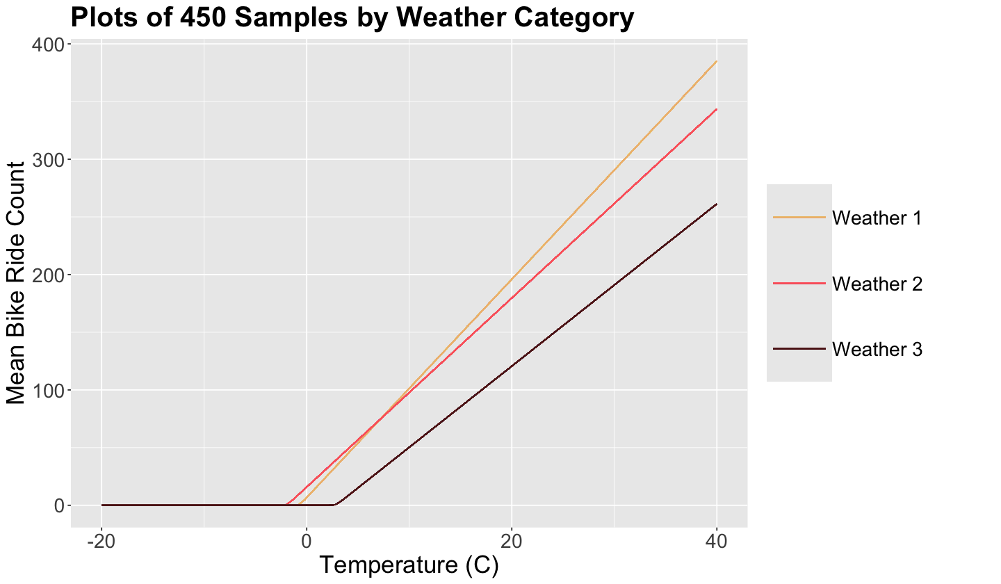
../_images/753829dd3b05cdafb60a3b9eb46a3f25d0cca6397066de760f55b77c34935562.png

The harshest weather 3 has the smallest slope and largest elbow. On the other hand, the nicest weather 1 has the largest slope but not the smallest elbow!

Exercise 14

Once we have estimated our Bayesian model, what do you think is the major drawback? Thus, how can we improve this model?

6. Wrapping Up#

We have built a Bayesian generative model totally from scratch by setting up key mathematical relations between our variables of interest.
Knowing the suitable class of distributions to use is of particular importance.
There is more than one possible modelling approach, and all models can be improved!

Lecture 4 - Markov Chain Monte Carlo, Stan, and Complex Bayesian Models

Contents

Lecture 4 - Markov Chain Monte Carlo, Stan, and Complex Bayesian Models#

Today’s Learning Objectives#

Loading R Packages#

Previously…#

1. The Big Idea#

1.1. To Design the Model, Think Generatively!#

1.2. Constructing the Likelihood#

2. The Bikeshare Data#

2.1. Data Wrangling#

2.2. Exploratory Data Analysis#

3. Bikeshare Likelihood#

3.1. Modelling the Bike Ride Counts#

3.2. Modelling the Weather Parameters#

4. Overview of Markov Chain Monte Carlo#

4.1. Monte Carlo Algorithm#

4.2. Markov Chain#

4.3. The Metropolis-Hastings Algorithm#

4.4. The Metropolis Algorithm#

4.5. Other MCMC Algorithms#

4.6. Important Facts to Consider when sampling() via rstan#

5. Using Stan to Obtain our Posterior Distribution#

5.1. Coding the Model#

5.2. MCMC Simulation#

5.3. Obtaining, Visualizing, and Interpreting the Posterior Results#

6. Wrapping Up#

Lecture 4 - Markov Chain Monte Carlo, `Stan`, and Complex Bayesian Models#

Loading `R` Packages#

4.6. Important Facts to Consider when `sampling()` via `rstan`#

5. Using `Stan` to Obtain our Posterior Distribution#