Lecture 7 - Bayesian Hierarchical Models

Lecture 7 - Bayesian Hierarchical Models#

Today’s Learning Objectives#

Explain the concept of the Bayesian hierarchical model.
Contrast the hierarchical model versus standard Bayesian models.
Demonstrate the advantages of hierarchical modelling in Bayesian inference.
Apply hierarchical modelling to predictive inquiries.

Loading `R` Packages#

options(repr.matrix.max.rows = 6)
library(tidyverse)
library(rstan)
library(broom.mixed)
library(bayesplot)
library(cowplot)
library(bayesrules)

Previously…#

We are in the last week of the block, and we have been exposed to standard Bayesian models. These models involve a likelihood conditioned on parameters of interest, which are random variables. These parameters have prior distributions. Furthermore, these priors have fixed hyperparameters.

Suppose you want to make inference on the mean number of people who stand in line, from 9:00 to 10:00 a.m. on Mondays, in the branches of a major Canadian bank. You collect data across different branches during that time slot and end up with $n$ observations. Moreover, you decide to take a Bayesian approach for this inquiry.

Nonetheless, we can make a flexible model in such a way we assign a mean by branch. Hence, let $S_i$ be the number of people standing in line from 9:00 to 10:00 a.m. on Mondays in the $i$th branch $(i = 1, \dots, n)$, and $\theta_i$ the mean by branch. Therefore, the formal Bayesian model will be the following:

\[\begin{split}\begin{align*} \text{likelihood:} \qquad S_i \mid \theta_i \mathop\sim^\text{ind} \text{Poisson}(\theta_i) \quad \text{for } i = 1, \dots, n \\ \text{priors:} \qquad \theta_i \sim \text{Gamma}(\alpha, \beta) \\ \qquad \alpha \sim \text{Exponential}(\eta = 0.1) \\ \qquad \beta \sim \text{Exponential}(\gamma = 0.5). \end{align*}\end{split}\]

Note $\alpha$ and $\beta$ are now random variables! This is a hierarchical model!

Exercise 19

Why do $\alpha$ and $\beta$ have Exponential priors?

A. Both $\alpha$ and $\beta$ are discrete and nonnegative in the Gamma prior distribution of $\theta_i$.

B. Both $\alpha$ and $\beta$ are continuous and unbounded in the Gamma prior distribution of $\theta_i$.

C. Both $\alpha$ and $\beta$ are continuous and nonnegative in the Gamma prior distribution of $\theta_i$.

D. Both $\alpha$ and $\beta$ are discrete and unbounded in the Gamma prior distribution of $\theta_i$.

1. The Rockets Data#

To illustrate the differences between the Bayesian models we have seen so far and the concept of hierarchy, we will retake the rockets problem from lab2. Then, throughout the lecture, we will build different Bayesian arrangements until we get to a hierarchical model. This will highlight these differences according to each model’s specific inferential inquiry.

Important

Recall rockets contains data on 367 rockets. It has three columns:

LV.Type: The rocket’s type.
numberOfLaunches: Number of launches.
numberOfFailures: Number of failures.

rockets <- read_csv("../data/failure_counts.csv", show_col_types = FALSE)
rockets

A spec_tbl_df: 367 × 3
LV.Type	numberOfLaunches	numberOfFailures
<chr>	<dbl>	<dbl>
Aerobee	1	0
Angara A5	1	0
Antares 110	2	0
⋮	⋮	⋮
Zenit-3SL	36	3
Zenit-3SLB	6	0
Zenit-3SLBF	3	0

2. Single Rocket Model (Warmup!)#

Let

\[X|\pi \sim \text{Binomial}(n,\pi)\]

be the number of successes that a specific rocket had in $n$ launches. We will assume that the probability of success $\pi$ is a continuous random variable that can take any value in the interval $[0, 1]$.

As our prior distribution, we will define a Beta PDF over the interval $[0, 1]$. Thus, the formal Bayesian model will be:

\[\begin{split}\begin{align*} \text{likelihood:} \qquad X|\pi \sim \text{Binomial}(n, \pi)\\ \text{prior:} \qquad \pi \sim \text{Beta}(a = 1,b = 1). \end{align*}\end{split}\]

Let us call it Single_Rocket.

Attention

For a GIVEN type of rocket (i.e., a row in rockets), our goal with Single_Rocket will be to infer its launch success probability $\pi$.

2.1. Coding the Model#

We start by coding Single_Rocket on Stan.

Single_Rocket <- "data {                          
int<lower=1> n;    // Number of trials in a given rocket type
int<lower=0> X;    // Number of successes in a given rocket type
real<lower=0> a;   // Hyperparameter for Beta prior
real<lower=0> b;   // Hyperparameter for Beta prior
}
parameters {
real <lower=0,upper=1> pi;    // Probability of launch success in a given rocket type 
}
model {
pi ~ beta(a, b);
X ~ binomial(n, pi);
}"

2.2. Running the MCMC Simulation#

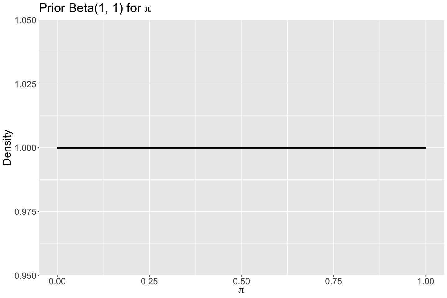
Suppose you are interested in making inference in the launch success probability $\pi$ for the type Ariane 1. Hence, let us use that row from rockets as our observed data. First, we create the data dictionary and proceed with stan(). We use a prior $\text{Beta}(a = 1, b = 1)$ which assumes all values of $\pi$ as equally probable.

options(repr.plot.height = 8, repr.plot.width = 12)

# Plotting Beta(1,1) prior
prior_beta_1_1 <- ggplot() +
  xlim(0, 1) +
  geom_function(fun = dbeta, args = list(shape1 = 1, shape2 = 1), linewidth = 2) +
  theme(
    plot.title = element_text(size = 24),
    axis.text.x = element_text(size = 17, angle = 0),
    axis.text.y = element_text(size = 17, angle = 0),
    axis.title = element_text(size = 21),
  ) +
  labs(y = "Density", x = expression(pi)) +
  ggtitle(expression(paste("Prior Beta(1, 1) for ", pi)))

prior_beta_1_1

../_images/67b7d55b5a99c027581e68cbf2827a8b879f5712c1f3e30dd956e04351d2a119.png

Ariane_1_data <- rockets |>
  filter(LV.Type == "Ariane 1")
Ariane_1_data

Single_Rocket_dictionary <- list(
  n = Ariane_1_data$numberOfLaunches, 
  X = Ariane_1_data$numberOfLaunches - Ariane_1_data$numberOfFailures, # Successes in Ariane 1
  a = 1, b = 1
)

A spec_tbl_df: 1 × 3
LV.Type	numberOfLaunches	numberOfFailures
<chr>	<dbl>	<dbl>
Ariane 1	11	2

posterior_Single_Rocket <- stan(
  model_code = Single_Rocket,
  data = Single_Rocket_dictionary,
  chains = 1,
  iter = 10000,
  warmup = 1000,
  thin = 5,
  seed = 553,
)

SAMPLING FOR MODEL 'anon_model' NOW (CHAIN 1).
Chain 1: 
Chain 1: Gradient evaluation took 4e-06 seconds
Chain 1: 1000 transitions using 10 leapfrog steps per transition would take 0.04 seconds.
Chain 1: Adjust your expectations accordingly!
Chain 1: 
Chain 1: 
Chain 1: Iteration:    1 / 10000 [  0%]  (Warmup)
Chain 1: Iteration: 1000 / 10000 [ 10%]  (Warmup)
Chain 1: Iteration: 1001 / 10000 [ 10%]  (Sampling)
Chain 1: Iteration: 2000 / 10000 [ 20%]  (Sampling)
Chain 1: Iteration: 3000 / 10000 [ 30%]  (Sampling)
Chain 1: Iteration: 4000 / 10000 [ 40%]  (Sampling)
Chain 1: Iteration: 5000 / 10000 [ 50%]  (Sampling)
Chain 1: Iteration: 6000 / 10000 [ 60%]  (Sampling)
Chain 1: Iteration: 7000 / 10000 [ 70%]  (Sampling)
Chain 1: Iteration: 8000 / 10000 [ 80%]  (Sampling)
Chain 1: Iteration: 9000 / 10000 [ 90%]  (Sampling)
Chain 1: Iteration: 10000 / 10000 [100%]  (Sampling)
Chain 1: 
Chain 1:  Elapsed Time: 0.002 seconds (Warm-up)
Chain 1:                0.017 seconds (Sampling)
Chain 1:                0.019 seconds (Total)
Chain 1: 

2.3. Output Summary#

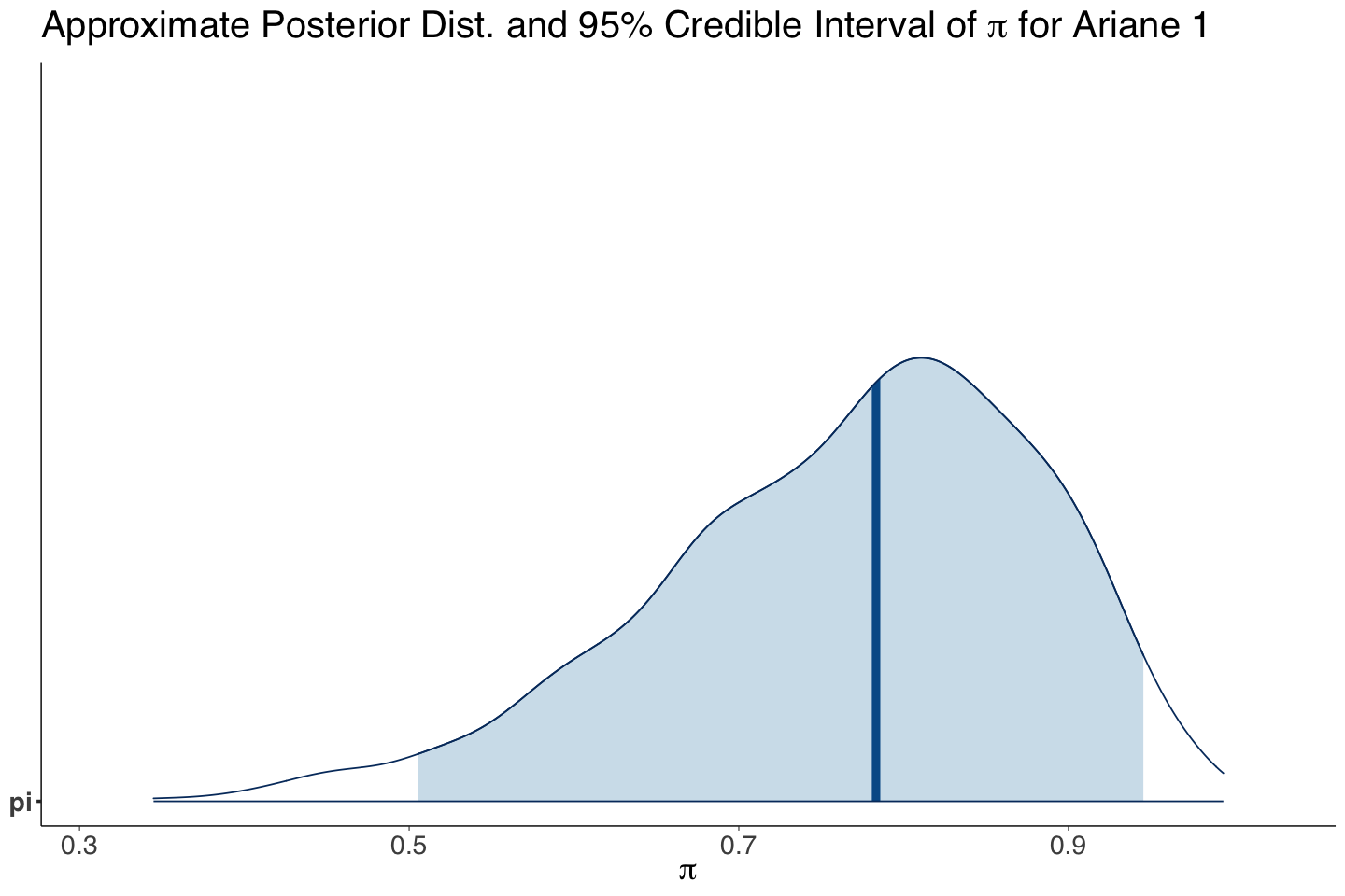
With a left-skewed distribution, our posterior mean of $\pi$ for Ariane 1 is 0.767. Moreover, the 95% credible interval shows high variability. Therefore, we could either increase our sample size for Ariane 1 (to have a narrower likelihood) or tune the Beta prior (i.e., a prior with less variability).

summary_Ariane_1 <- as.data.frame(summary(posterior_Single_Rocket)$summary)
summary_Ariane_1 <- summary_Ariane_1[1, c("mean", "sd", "2.5%", "97.5%")] %>%
  mutate_if(is.numeric, round, 3)
summary_Ariane_1

A data.frame: 1 × 4
	mean	sd	2.5%	97.5%
	<dbl>	<dbl>	<dbl>	<dbl>
pi	0.767	0.116	0.505	0.945

post_plot_Ariane_1 <- mcmc_areas(posterior_Single_Rocket, pars = "pi", prob = 0.95) +
  theme(
    plot.title = element_text(size = 24, family = "sans"),
    axis.text.x = element_text(size = 17, angle = 0, family = "sans"),
    axis.text.y = element_text(size = 17, angle = 0, family = "sans"),
    axis.title = element_text(size = 21, family = "sans")
  ) +
  labs(title = expression(paste("Approximate Posterior Dist. and 95% Credible Interval of ", pi, " for Ariane 1"))) +
  xlab(expression(pi))

post_plot_Ariane_1

../_images/78797e762742c5c0b8a5ac2a792b2e51fbd553c1e8e7cea999630d7df38d15a0.png

3. Complete Pooled Rocket Model#

Our second Bayesian approach is called a complete pooled model. In this model, we will combine the data provided by ALL rockets into one pool of information. For the $i$th rocket, the model is:

\[\begin{split}\begin{align*} \text{likelihood:} \qquad X_i|\pi \sim \text{Binomial}(n_i, \pi) \quad \text{for } i = 1, \dots, 367\\ \text{prior:} \qquad \pi \sim \text{Beta}(a = 1, b = 1). \end{align*}\end{split}\]

Caution

Even though it might not look like it, this model is quite different from the SingleRocket model. The difference is that, in this complete pooled model, we are considering all the rocket types.

While we allow them to have different numbers of launches, we assume that all of them have the same probability of success $\pi$. In this way, we will be estimating the OVERALL probability of success across all rockets.

3.1. Coding the Model#

We code up this Complete_Pooled_Rocket model on Stan. Note the data block includes one integer to define the number of rockets to use in the simulation (num_rockets), a vector of integers containing all launch successes by rocket (X[num_rockets]), and a vector of integers containing all trials by rocket (n[num_rockets]).

Complete_Pooled_Rocket <- "data {                          
int<lower=1> num_rockets;     // number of rockets 
int<lower=0> X[num_rockets];  // vector with sucesses by rocket
int<lower=1> n[num_rockets];  // vector with trials by rocket
real<lower=0> a;
real<lower=0> b;  
}
parameters {
real <lower=0,upper=1> pi;
}
model {
pi ~ beta(a, b);
for (i in 1:num_rockets){    // modelling the likelihood by rocket
X[i] ~ binomial(n[i], pi);
}
}"

3.2. Running the MCMC Simulation#

To build the Complete_Pooled_Rocket_dictionary we need to use the corresponding columns from rockets. Recall X is provided by substracting two columns.

Complete_Pooled_Rocket_dictionary <- list(
  num_rockets = nrow(rockets),
  X = rockets$numberOfLaunches - rockets$numberOfFailures,
  n = rockets$numberOfLaunches,
  a = 1, b = 1
)

posterior_Complete_Pooled_Rocket <- stan(
  model_code = Complete_Pooled_Rocket,
  data = Complete_Pooled_Rocket_dictionary,
  chains = 1,
  iter = 10000,
  warmup = 1000,
  thin = 5,
  seed = 553,
)

SAMPLING FOR MODEL 'anon_model' NOW (CHAIN 1).
Chain 1: 
Chain 1: Gradient evaluation took 2.2e-05 seconds
Chain 1: 1000 transitions using 10 leapfrog steps per transition would take 0.22 seconds.
Chain 1: Adjust your expectations accordingly!
Chain 1: 
Chain 1: 
Chain 1: Iteration:    1 / 10000 [  0%]  (Warmup)
Chain 1: Iteration: 1000 / 10000 [ 10%]  (Warmup)
Chain 1: Iteration: 1001 / 10000 [ 10%]  (Sampling)
Chain 1: Iteration: 2000 / 10000 [ 20%]  (Sampling)
Chain 1: Iteration: 3000 / 10000 [ 30%]  (Sampling)
Chain 1: Iteration: 4000 / 10000 [ 40%]  (Sampling)
Chain 1: Iteration: 5000 / 10000 [ 50%]  (Sampling)
Chain 1: Iteration: 6000 / 10000 [ 60%]  (Sampling)
Chain 1: Iteration: 7000 / 10000 [ 70%]  (Sampling)
Chain 1: Iteration: 8000 / 10000 [ 80%]  (Sampling)
Chain 1: Iteration: 9000 / 10000 [ 90%]  (Sampling)
Chain 1: Iteration: 10000 / 10000 [100%]  (Sampling)
Chain 1: 
Chain 1:  Elapsed Time: 0.06 seconds (Warm-up)
Chain 1:                0.451 seconds (Sampling)
Chain 1:                0.511 seconds (Total)
Chain 1: 

3.3. Output Summary#

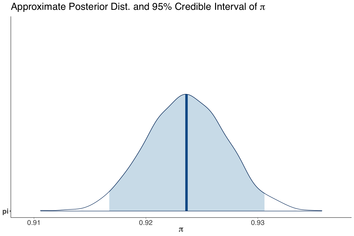
Unlike Ariane 1, the posterior distribution of the overall $\pi$ is symmetric with a mean of 0.924. Moreover, the 95% CI shows a low variability in this posterior distribution.

summary_Complete_Pooled_Rocket <- as.data.frame(summary(posterior_Complete_Pooled_Rocket)$summary)
summary_Complete_Pooled_Rocket <- summary_Complete_Pooled_Rocket[1, c("mean", "sd", "2.5%", "97.5%")] %>%
  mutate_if(is.numeric, round, 3)
summary_Complete_Pooled_Rocket

A data.frame: 1 × 4
	mean	sd	2.5%	97.5%
	<dbl>	<dbl>	<dbl>	<dbl>
pi	0.924	0.004	0.917	0.931

post_plot_Complete_Pooled_Rocket <- mcmc_areas(posterior_Complete_Pooled_Rocket, pars = "pi", prob = 0.95) +
  theme(
    plot.title = element_text(size = 24, family = "sans"),
    axis.text.x = element_text(size = 17, angle = 0, family = "sans"),
    axis.text.y = element_text(size = 17, angle = 0, family = "sans"),
    axis.title = element_text(size = 21, family = "sans")
  ) +
  labs(title = expression(paste("Approximate Posterior Dist. and 95% Credible Interval of ", pi))) +
  xlab(expression(pi))

post_plot_Complete_Pooled_Rocket

../_images/024e739da58c74ad1ab8cbc8c31652595fd1ebf9754901a662b4b926185f4d13.png

Exercise 20

Note that the approximate 95% credible interval for $\pi$ is $(0.917, 0.931)$. Is this interval an indicator of high precision on the estimation of $\pi$?

A. Yes.

B. No.

4. Let Us Go to Space!#

You told a certain CEO from a rocket company that you wanted to go to space, and they asked you to pick your preferred rocket model from the rockets dataset. Let us try to decide which rocket we trust the most. Therefore, the Bayesian Complete_Pooled_Rocket is not suitable for this purpose since it makes inference on a single $\pi$!

We will start with a similar approach such as in lab1 for the helicopter problem.

Firstly, we will only trust our observed data (i.e., the likelihood) without relying on the Bayes’ rule. This will implicate using maximum likelihood estimation to compute $\hat{\pi}_i$ for the $i$th rocket $(i = 1, \dots, 367)$. In a Binomial likelihood, we know the maximum likelihood estimate (MLE) is:

\[\hat{\pi}_i = \frac{x_i}{n_i},\]

where $x_i$ and $n_i$ are the respective observed numbers of successes and trials.

We will compute $\hat{\pi}_i$ in rockets so we can select that rocket with the largest estimation for its launch success probability.

options(repr.matrix.max.rows = 60)

rockets <- rockets |>
  mutate(MLE = (numberOfLaunches - numberOfFailures) / numberOfLaunches)

rockets |>
  arrange(-MLE, LV.Type)

A tibble: 367 × 4
LV.Type	numberOfLaunches	numberOfFailures	MLE
<chr>	<dbl>	<dbl>	<dbl>
ARPA Taurus	2	0	1
Aerobee	1	0	1
Angara A5	1	0	1
Antares 110	2	0	1
Antares 120	2	0	1
Antares 230	1	0	1
Ariane 40	7	0	1
Ariane 42L	13	0	1
Ariane 44P	15	0	1
Ariane 5ES	1	0	1
Ariane 5ES/ATV	5	0	1
Ariane 5G+	3	0	1
Ariane 5GS	6	0	1
Athena-1	2	0	1
Atlas 3A	2	0	1
Atlas 3B	4	0	1
Atlas Agena D	15	0	1
Atlas B	1	0	1
Atlas Centaur D	7	0	1
Atlas E	15	0	1
Atlas E Altair	1	0	1
Atlas E/OIS	1	0	1
Atlas E/SGS-2	4	0	1
Atlas F/Agena D	1	0	1
Atlas F/MSD	3	0	1
Atlas F/OIS	1	0	1
Atlas F/PTS	1	0	1
Atlas F/SVS	7	0	1
Atlas H	5	0	1
Atlas II	10	0	1
⋮	⋮	⋮	⋮
Proton-M/DM-3	3	2	0.3333333
Scout X-2M	3	2	0.3333333
Thor Able I	3	2	0.3333333
Vostok-L 8K72	9	6	0.3333333
Vanguard	11	8	0.2727273
Lambda 4S	5	4	0.2000000
Antares 130	1	1	0.0000000
Atlas Able	3	3	0.0000000
Atlas E/MSD	1	1	0.0000000
Atlas E/SVS	1	1	0.0000000
Blue Scout II	1	1	0.0000000
Chang Zheng 2	1	1	0.0000000
Conestoga 1620	1	1	0.0000000
Energiya	1	1	0.0000000
Europa I	3	3	0.0000000
Europa II	1	1	0.0000000
KT-1	3	3	0.0000000
LLV-1	1	1	0.0000000
N-1 11A52	4	4	0.0000000
Paektusan 1	1	1	0.0000000
Project Pilot	6	6	0.0000000
SS-520	1	1	0.0000000
Scout X-2B	1	1	0.0000000
Start	1	1	0.0000000
Super Strypi	1	1	0.0000000
Taurus 3110	2	2	0.0000000
Unha-2	1	1	0.0000000
VLS-1	2	2	0.0000000
Volna	1	1	0.0000000
Zenit-2 11K77.05	1	1	0.0000000

We can see there is more than one rocket with a 100% success rate! Nevertheless, they often could have a small number of launches. So we might not trust those rockets all that much. MLE is frequentist-based; thus, it heavily relies on large sample sizes!

Bayesian inference can help us decide while considering sample size by rocket with the upcoming model.

5. Non-Pooled Rocket Model#

Our third Bayesian approach is a non-pooled model. In this model, we will make inference on the 367 different success probabilities (one by rocket) in a single Stan model. This approach goes to the other extreme when compared to Complete_Pooled_Rocket!

For the $i$th rocket, the model is:

\[\begin{split}\begin{align*} \text{likelihood:} \qquad X_i|\pi_i \sim \text{Binomial}(n_i, \pi_i) \quad \text{for } i = 1, \dots, 367\\ \text{prior:} \qquad \pi_i \sim \text{Beta}(a = 1,b = 1). \end{align*}\end{split}\]

Exercise 21

In this non-pooled model, is it possible to make inference on an overall $\pi$?

A. Yes.

B. No.

5.1. Coding the Model#

We code up this Non_Pooled_Rocket model on Stan. The data block structure from Complete_Pooled_Rocket remains. However, we tweak the model block to assign the same prior beta(a,b) by rocket probability. Furthermore, the parameters block is adapted to have a vector of probabilities pi of size num_rockets.

Non_Pooled_Rocket <- "data {                          
int<lower=1> num_rockets;     // number of rockets 
int<lower=0> X[num_rockets];  // vector with sucesses by rocket
int<lower=1> n[num_rockets];  // vector with trials by rocket
real<lower=0> a;
real<lower=0> b;  
}
parameters {
vector<lower=0,upper=1>[num_rockets] pi;  // vector of 367 probabilities of success (one per rocket)
}
model {
for (i in 1:num_rockets){
pi[i] ~ beta(a,b);           // prior for pi_i by rocket
X[i] ~ binomial(n[i],pi[i]); // modelling the likelihood by rocket
}
}"

5.2. Running the MCMC Simulation#

To run the Non_Pooled_Rocket model, we need to use the corresponding columns from rockets. The dictionary is identical to Complete_Pooled_Rocket_dictionary.

Non_Pooled_Rocket_dictionary <- list(
  num_rockets = nrow(rockets),
  X = rockets$numberOfLaunches - rockets$numberOfFailures,
  n = rockets$numberOfLaunches,
  a = 1, b = 1
)

posterior_Non_Pooled_Rocket <- stan(
  model_code = Non_Pooled_Rocket,
  data = Non_Pooled_Rocket_dictionary,
  chains = 1,
  iter = 10000,
  warmup = 1000,
  thin = 5,
  seed = 553,
)

SAMPLING FOR MODEL 'anon_model' NOW (CHAIN 1).
Chain 1: 
Chain 1: Gradient evaluation took 8.3e-05 seconds
Chain 1: 1000 transitions using 10 leapfrog steps per transition would take 0.83 seconds.
Chain 1: Adjust your expectations accordingly!
Chain 1: 
Chain 1: 
Chain 1: Iteration:    1 / 10000 [  0%]  (Warmup)
Chain 1: Iteration: 1000 / 10000 [ 10%]  (Warmup)
Chain 1: Iteration: 1001 / 10000 [ 10%]  (Sampling)
Chain 1: Iteration: 2000 / 10000 [ 20%]  (Sampling)
Chain 1: Iteration: 3000 / 10000 [ 30%]  (Sampling)
Chain 1: Iteration: 4000 / 10000 [ 40%]  (Sampling)
Chain 1: Iteration: 5000 / 10000 [ 50%]  (Sampling)
Chain 1: Iteration: 6000 / 10000 [ 60%]  (Sampling)
Chain 1: Iteration: 7000 / 10000 [ 70%]  (Sampling)
Chain 1: Iteration: 8000 / 10000 [ 80%]  (Sampling)
Chain 1: Iteration: 9000 / 10000 [ 90%]  (Sampling)
Chain 1: Iteration: 10000 / 10000 [100%]  (Sampling)
Chain 1: 
Chain 1:  Elapsed Time: 1.194 seconds (Warm-up)
Chain 1:                7.645 seconds (Sampling)
Chain 1:                8.839 seconds (Total)
Chain 1: 

5.3. Output Summary#

We obtain the output from Non_Pooled_Rocket. Since Stan labels the parameters in the posterior samples as pi[1], …, pi[367], we will add a new column with the actual rocket name using rockets$LV.Type.

options(repr.matrix.max.rows = 15)

summary_Non_Pooled_Rocket <- as.data.frame(summary(posterior_Non_Pooled_Rocket)$summary)
summary_Non_Pooled_Rocket <- summary_Non_Pooled_Rocket[-368, c("mean", "sd", "2.5%", "97.5%")] |>
  mutate_if(is.numeric, round, 3)
summary_Non_Pooled_Rocket$rocket <- rockets$LV.Type
summary_Non_Pooled_Rocket |>
  arrange(-mean)

A data.frame: 367 × 5
	mean	sd	2.5%	97.5%	rocket
	<dbl>	<dbl>	<dbl>	<dbl>	<chr>
pi[266]	0.987	0.013	0.953	1.000	Soyuz-U2
pi[267]	0.985	0.011	0.959	0.998	Space Shuttle
pi[261]	0.984	0.016	0.941	0.999	Soyuz-FG
pi[357]	0.978	0.015	0.942	0.997	Vostok 8A92M
pi[343]	0.972	0.016	0.934	0.994	Tsiklon-2
pi[78]	0.971	0.029	0.894	1.000	Chang Zheng 2D
pi[264]	0.970	0.007	0.955	0.982	Soyuz-U
pi[16]	0.969	0.021	0.916	0.996	Ariane 5ECA
⋮	⋮	⋮	⋮	⋮	⋮
pi[281]	0.255	0.196	0.009	0.711	Taurus 3110
pi[353]	0.250	0.188	0.009	0.692	VLS-1
pi[28]	0.204	0.167	0.006	0.623	Atlas Able
pi[179]	0.203	0.165	0.008	0.601	KT-1
pi[157]	0.201	0.161	0.006	0.589	Europa I
pi[201]	0.165	0.140	0.005	0.507	N-1 11A52
pi[211]	0.125	0.113	0.003	0.422	Project Pilot

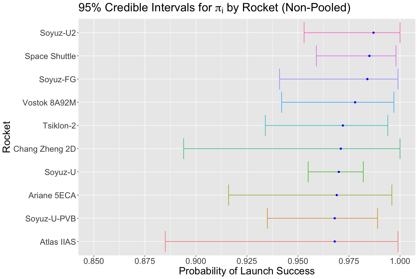
Note that the top 3 rockets in the posterior values for $\pi_i$ do not correspond to the previous top 3 rockets in MLE from rockets. We can also plot the top 10 rockets by posterior mean probability of launch and the 95% credible intervals. Note the overlap across these ten rockets.

posterior_rocket_CIs_plot_Non_Pooled <- summary_Non_Pooled_Rocket |>
  arrange(-mean) |>
  slice(1:10) |>
  mutate(rocket = fct_reorder(rocket, mean)) |>
  ggplot(aes(x = mean, y = rocket)) +
  geom_errorbarh(aes(xmax = `2.5%`, xmin = `97.5%`, color = rocket)) +
  geom_point(color = "blue") +
  theme(
    plot.title = element_text(size = 24),
    axis.text = element_text(size = 17),
    axis.title = element_text(size = 21),
    legend.position = "none"
  ) +
  ggtitle(expression(paste("95% Credible Intervals for ", pi[i], " by Rocket (Non-Pooled)"))) +
  labs(x = "Probability of Launch Success", y = "Rocket") +
  scale_x_continuous(limits=c(0.85, 1), breaks = seq(0.85, , 0.025))

posterior_rocket_CIs_plot_Non_Pooled

../_images/359c928008e71d3b08960f4565479516c44cd96a0590180e767e75f5d3ed3576.png

Let us add our Bayesian posterior means to rockets and sort them from the largest posterior mean to the lowest.

options(repr.matrix.max.rows = 20)
rockets$posterior_non_pooled_means <- summary_Non_Pooled_Rocket$mean
rockets |>
  arrange(-posterior_non_pooled_means)

A tibble: 367 × 5
LV.Type	numberOfLaunches	numberOfFailures	MLE	posterior_non_pooled_means
<chr>	<dbl>	<dbl>	<dbl>	<dbl>
Soyuz-U2	72	0	1.0000000	0.987
Space Shuttle	135	1	0.9925926	0.985
Soyuz-FG	59	0	1.0000000	0.984
Vostok 8A92M	93	1	0.9892473	0.978
Tsiklon-2	105	2	0.9809524	0.972
Chang Zheng 2D	32	0	1.0000000	0.971
Soyuz-U	633	18	0.9715640	0.970
Ariane 5ECA	61	1	0.9836066	0.969
Atlas IIAS	30	0	1.0000000	0.968
Soyuz-U-PVB	154	4	0.9740260	0.968
⋮	⋮	⋮	⋮	⋮
Zenit-2 11K77.05	1	1	0.0000000	0.328
Vanguard	11	8	0.2727273	0.310
Lambda 4S	5	4	0.2000000	0.287
Taurus 3110	2	2	0.0000000	0.255
VLS-1	2	2	0.0000000	0.250
Atlas Able	3	3	0.0000000	0.204
KT-1	3	3	0.0000000	0.203
Europa I	3	3	0.0000000	0.201
N-1 11A52	4	4	0.0000000	0.165
Project Pilot	6	6	0.0000000	0.125

Exercise 22

From rockets, which one of the two estimators (MLE or the posterior mean with Non_Pooled_Rocket) do you think is more helpful in choosing your rocket?

6. Hierarchical Rocket Model#

Except for the initial warmup model (which is a single iteration of Non_Pooled_Rocket!), we have tried different Bayesian models using two opposite approaches:

Complete_Pooled_Rocket: We obtained approximate posterior samples for $\pi$, the overall probability of launch success. However, this approach does not allow us to infer any probability of an individual rocket.
Non_Pooled_Rocket: We obtained approximate posterior samples for the probability of launch success $\pi_i$ by EACH rocket type.

To choose the most successful rocket, Non_Pooled_Rocket worked reasonably better than MLE. However, recall the formal modelling:

\[\begin{split}\begin{align*} \text{likelihood:} \qquad X_i|\pi_i \sim \text{Binomial}(n_i, \pi_i) \quad \text{for } i = 1, \dots, 367\\ \text{prior:} \qquad \pi_i \sim \text{Beta}(a = 1, b = 1). \end{align*}\end{split}\]

Caution

Why should we restrict our prior for each $\pi_i$ to fixed hyperparameters $a$ and $b$ for the Beta distribution? We have only been using $\text{Beta}(a = 1, b = 1)$ thorughout the whole lecture!

There are other important drawbacks in Non_Pooled_Rocket:

Firstly, we cannot generalize this model to some new rocket.
Secondly, we would not take any valuable information provided by some rocket type to infer on another type in rockets.

Here comes another Bayesian twist! To make the model even more flexible, let us make $a$ and $b$ random too in the Beta prior. Hence, $a$ and $b$ will become parameters too (and not hyperparameters!).

Important

This is the foundational point of a hierarchical model. This hierarchical model will take into account two sources of variability (different to the predictive sources of variability we saw in Lecture 5 - Bayesian Normal Linear Regression and Hypothesis Testing):

Within-group variability: How much variability we have among the observations within each group of interest. In this case, the group is a rocket type, while the observations are different trials.
Between-group variability: How much variability we have from group to group. In this example, we can assess this matter from one rocket type to another.

Essentially, the hierarchical model takes the best of Non_Pooled_Rocket and Complete_Pooled_Rocket. Note it will be able to infer on the following:

It will use valuable information from all the rockets in the dataset to infer the launch success probability on a specific rocket.
We can obtain the posterior predictive distribution of the launch success probability for a new rocket.

Our hierarchical model is formally defined as:

\[\begin{split}\begin{align*} \text{likelihood:} \qquad X_i|\pi_i \sim \text{Binomial}(n_i, \pi_i) \quad \text{for } i = 1, \dots, 367\\ \text{priors:} \qquad \pi_i \sim \text{Beta}(a, b) \\ \quad a \sim \text{Gamma}(0.001, 0.001) \\ \qquad b \sim \text{Gamma}(0.001, 0.001). \end{align*}\end{split}\]

What is the big picture here?

First, this hierarchical model learns a different $\pi_i$ from each rocket type. The key here is that the data from all rockets contribute to our inferences about $a$ and $b$. Thus, it is like our prior for each rocket is being set by all the rockets!

6.1. The Priors#

Why a Gamma distribution for $a$ and $b$?

Recall the probability density function (PDF) of the Beta distribution:

\[f(\pi_i) = \frac{\Gamma(a + b)}{\Gamma(a) \Gamma(b)} \pi_i ^{a - 1} (1 - \pi_i)^{b - 1} \quad \text{for} \quad 0 \leq \pi_i \leq 1.\]

In this PDF, we have that $a > 0$ and $b > 0$ are continuous. Thus, a nonnegative continuous Gamma is suitable in this case.

# Plotting Gamma prior
prior_gamma <- ggplot() +
  xlim(0, 10) +
  ylim(0, 10) +
  geom_function(fun = dgamma, args = list(shape = 0.001, rate = 0.001), linewidth = 2) +
  geom_vline(xintercept = 0.00001, colour = "darkred", linetype = "dashed", linewidth = 2) +
  theme(
    plot.title = element_text(size = 24, face = "bold"),
    axis.text.x = element_text(size = 17, angle = 0),
    axis.text.y = element_text(size = 17, angle = 0),
    axis.title = element_text(size = 21),
  ) +
  labs(y = "Density", x = "Hierarchical Parameter") +
  ggtitle("Prior Gamma(0.001, 0.001) for a and b" )

The corresponding Gamma prior distribution for $a$ and $b$ are plotted below (the prior mean is the vertical dashed red line).

prior_gamma

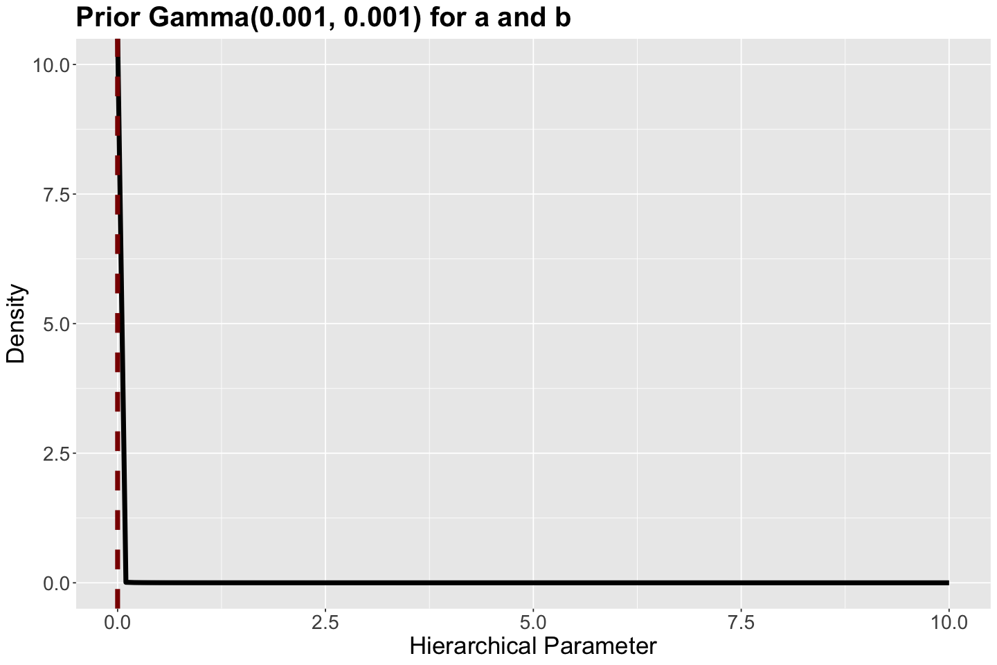
../_images/77b36ab1a677c3c13ddecfba7b30a92fd6d17c5fc6ee84013c2f053b274b16b1.png

Note the Gamma priors tend to assign small values for $a$ and $b$ in

\[\pi_i \sim \text{Beta}(a, b).\]

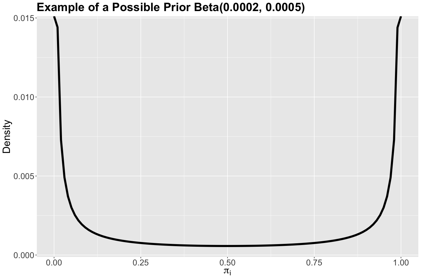
As an example, for a given $\pi_i$, suppose its Beta prior has $a = 0.0002$ and $b = 0.0005$. This Beta prior for $\pi_i$ is plotted below. We can see these prior beliefs for $a$ and $b$ basically put the success probability $\pi_i$ close to either its lower or upper bound. Translating this into our prior beliefs, we think that any rocket would be either good or bad (we do not want any intermediate point here since we are using that rocket to go to space!).

# Plotting Beta prior
prior_beta <- ggplot() +
  xlim(0, 1) +
  geom_function(fun = dbeta, args = list(shape1 = 0.0002, shape2 = 0.0005), linewidth = 2) +
  theme(
    plot.title = element_text(size = 24, face = "bold"),
    axis.text.x = element_text(size = 17, angle = 0),
    axis.text.y = element_text(size = 17, angle = 0),
    axis.title = element_text(size = 21),
  ) +
  labs(y = "Density", x = expression(pi["i"])) +
  ggtitle("Example of a Possible Prior Beta(0.0002, 0.0005)")

prior_beta

../_images/0b700aad5e0797fd29a7ae2294ba839a66bbc09d04ab8f8450cd7aa1499ad735.png

6.2. Coding the Model#

We code up this Hierarchical_Rocket model on Stan:

The data block structure will not have a and b since they are random now.
Furthermore, we add the Gamma priors for $a$ and $b$ in the model block while keeping the Beta prior for each $\pi_i$.
The parameters block has new variables: a and b.
Besides the posterior sampled probabilities by rocket type, we will also obtain posterior samples for $a$ and $b$.

Hierarchical_Rocket <- "data {                          
int<lower=1> num_rockets;    // number of rockets 
int<lower=0> X[num_rockets];  // vector with sucesses by rocket
int<lower=1> n[num_rockets];  // vector with trials by rocket
}
parameters {
vector<lower=0,upper=1>[num_rockets] pi; // vector of 367 probabilities of launch success
real<lower=0> a; // beta parameter
real<lower=0> b; // beta parameter
}
model {
a ~ gamma(0.001, 0.001);     // prior for a
b ~ gamma(0.001, 0.001);     // prior for b

for (i in 1:num_rockets){
pi[i] ~ beta(a,b);           // modelling the pi_i by rocket
X[i] ~ binomial(n[i],pi[i]); // modelling the likelihood by rocket
}
}"

6.3. Running the MCMC Simulation#

To run the Hierarchical_Rocket model, we need to use the corresponding columns from rockets. This dictionary will not have a and b.

Hierarchical_Rocket_dictionary <- list(
  num_rockets = nrow(rockets),
  X = rockets$numberOfLaunches - rockets$numberOfFailures,
  n = rockets$numberOfLaunches
)

posterior_Hierarchical_Rocket <- stan(
  model_code = Hierarchical_Rocket,
  data = Hierarchical_Rocket_dictionary,
  chains = 1,
  iter = 10000,
  warmup = 1000,
  thin = 5,
  seed = 553,
)

SAMPLING FOR MODEL 'anon_model' NOW (CHAIN 1).
Chain 1: 
Chain 1: Gradient evaluation took 7e-05 seconds
Chain 1: 1000 transitions using 10 leapfrog steps per transition would take 0.7 seconds.
Chain 1: Adjust your expectations accordingly!
Chain 1: 
Chain 1: 
Chain 1: Iteration:    1 / 10000 [  0%]  (Warmup)
Chain 1: Iteration: 1000 / 10000 [ 10%]  (Warmup)
Chain 1: Iteration: 1001 / 10000 [ 10%]  (Sampling)
Chain 1: Iteration: 2000 / 10000 [ 20%]  (Sampling)
Chain 1: Iteration: 3000 / 10000 [ 30%]  (Sampling)
Chain 1: Iteration: 4000 / 10000 [ 40%]  (Sampling)
Chain 1: Iteration: 5000 / 10000 [ 50%]  (Sampling)
Chain 1: Iteration: 6000 / 10000 [ 60%]  (Sampling)
Chain 1: Iteration: 7000 / 10000 [ 70%]  (Sampling)
Chain 1: Iteration: 8000 / 10000 [ 80%]  (Sampling)
Chain 1: Iteration: 9000 / 10000 [ 90%]  (Sampling)
Chain 1: Iteration: 10000 / 10000 [100%]  (Sampling)
Chain 1: 
Chain 1:  Elapsed Time: 1.944 seconds (Warm-up)
Chain 1:                12.514 seconds (Sampling)
Chain 1:                14.458 seconds (Total)
Chain 1: 

6.4. Output Summary#

We obtain the output from posterior_Hierarchical_Rocket. Since Stan labels the parameters in the posterior samples as pi[1], …, pi[367], we will add a new column with the actual rocket name using rockets$LV.Type.

options(repr.matrix.max.rows = 12)
summary_Hierarchical_Rocket <- as.data.frame(summary(posterior_Hierarchical_Rocket)$summary)
summary_Hierarchical_Rocket <- summary_Hierarchical_Rocket[1:367, c("mean", "sd", "2.5%", "97.5%")] |>
  mutate_if(is.numeric, round, 3)
summary_Hierarchical_Rocket$rocket <- rockets$LV.Type
summary_Hierarchical_Rocket |>
  arrange(-mean)

A data.frame: 367 × 5
	mean	sd	2.5%	97.5%	rocket
	<dbl>	<dbl>	<dbl>	<dbl>	<chr>
pi[266]	0.991	0.011	0.961	1.000	Soyuz-U2
pi[261]	0.989	0.013	0.956	1.000	Soyuz-FG
pi[267]	0.988	0.010	0.963	0.999	Space Shuttle
pi[357]	0.983	0.013	0.950	0.998	Vostok 8A92M
pi[78]	0.982	0.021	0.923	1.000	Chang Zheng 2D
pi[54]	0.980	0.023	0.915	1.000	Atlas IIAS
⋮	⋮	⋮	⋮	⋮	⋮
pi[192]	0.545	0.074	0.398	0.685	Molniya 8K78
pi[184]	0.544	0.155	0.241	0.821	Lambda 4S
pi[360]	0.529	0.125	0.284	0.759	Vostok-L 8K72
pi[201]	0.496	0.162	0.187	0.800	N-1 11A52
pi[351]	0.470	0.123	0.242	0.701	Vanguard
pi[211]	0.405	0.145	0.147	0.699	Project Pilot

We plot the top 10 rockets and the posterior 95% credible intervals from posterior_Hierarchical_Rocket. Then we compare this top 10 versus the ones obtained with posterior_Non_Pooled_Rocket. The credible interval overlapping is still there.

Nonetheles, for those rockets still present in the top 10 from posterior_Hierarchical_Rocket, the credible intervals are narrower! We have more precise results.

posterior_rocket_CIs_plot_Hierarchical <- summary_Hierarchical_Rocket |>
  arrange(-mean) |>
  slice(1:10) |>
  mutate(rocket = fct_reorder(rocket, mean)) |>
  ggplot(aes(x = mean, y = rocket)) +
  geom_errorbarh(aes(xmax = `2.5%`, xmin = `97.5%`, color = rocket)) +
  geom_point(color = "blue") +
  theme(
    plot.title = element_text(size = 24),
    axis.text = element_text(size = 17),
    axis.title = element_text(size = 21),
    legend.position = "none"
  ) +
  ggtitle(expression(paste("95% Credible Intervals for ", pi[i], " by Rocket (Hierarchical)"))) +
  labs(x = "Probability of Launch Success", y = "Rocket") +
  scale_x_continuous(limits = c(0.85, 1), breaks = seq(0.85, , 0.025))

options(repr.plot.height = 11, repr.plot.width = 12)

plot_grid(posterior_rocket_CIs_plot_Non_Pooled, posterior_rocket_CIs_plot_Hierarchical, nrow = 2)

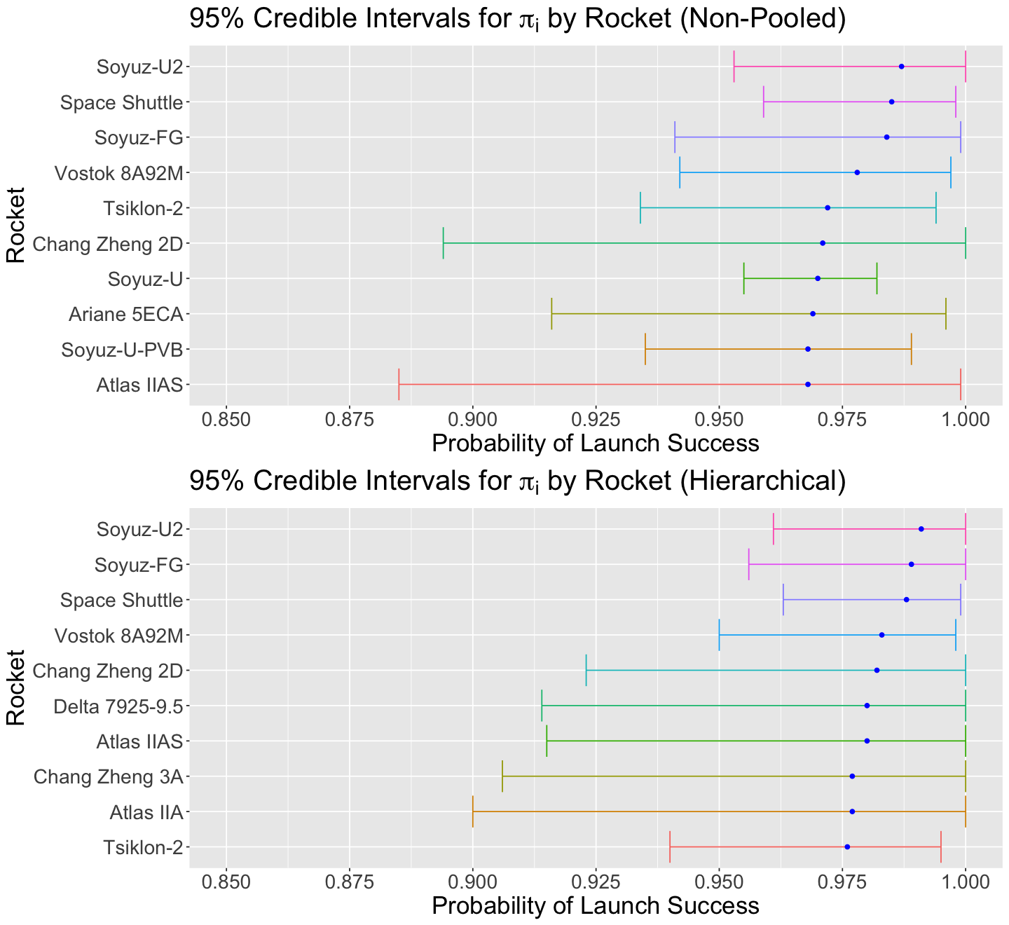
../_images/005e97909c3868c54977d37c3eea94277a72254e22fbd50704096e6586bab463.png

So, what rocket should we choose with a hierarchical model?

If we had to choose based on the hierarchical Bayesian results, we would still take Soyuz-U2 or Space Shuttle (now with narrower 95% credible intervals!).

Why are our estimates more precise?

A useful property of hierarchical models is the notion of “borrowing strength”, where a rocket uses the information about the probability of success from other rockets. As we saw above, this affects the mean of our posterior distributions, but it also affects the variance. This helps us to learn the parameters and actually reduce the posterior variance of our Bayesian estimates!

How about the posterior results for $a$ and $b$?

Also, we have posterior summaries for a and b.

summary_Hierarchical_Rocket_ab <- as.data.frame(summary(posterior_Hierarchical_Rocket)$summary)
summary_Hierarchical_Rocket_ab <- summary_Hierarchical_Rocket_ab[368:369, c("mean", "sd", "2.5%", "97.5%")] |>
  mutate_if(is.numeric, round, 3)
summary_Hierarchical_Rocket_ab

A data.frame: 2 × 4
	mean	sd	2.5%	97.5%
	<dbl>	<dbl>	<dbl>	<dbl>
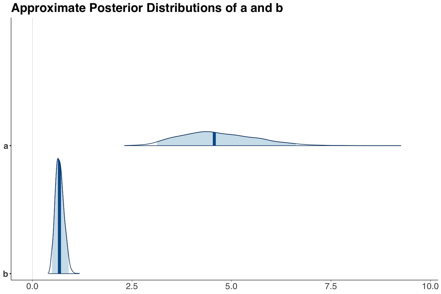
a	4.673	0.933	3.133	6.616
b	0.685	0.109	0.490	0.911

Note the posterior distributions of $a$ and $b$ are right-skewed.

post_plot_Hierarchical_Rocket_ab <- mcmc_areas(posterior_Hierarchical_Rocket, pars = c("a", "b"), prob = 0.95) +
  theme(
    plot.title = element_text(size = 24, face = "bold", family = "sans"),
    axis.text.x = element_text(size = 17, angle = 0, family = "sans"),
    axis.text.y = element_text(size = 17, angle = 0, family = "sans"),
    axis.title = element_text(size = 21, family = "sans"),
    strip.text.x = element_text(size = 17, family = "sans")
  ) +
  ggtitle("Approximate Posterior Distributions of a and b")

options(repr.plot.height = 8, repr.plot.width = 12)

post_plot_Hierarchical_Rocket_ab

../_images/c018056eb245976b56af1d50f03e540c8f82c17383857980ed85f8068e6e95fd.png

How is the average launch success probability for all the rockets?

We will use the posterior means of $a$ and $b$ as parameters of a Beta distribution to report posterior metrics on the average launch probability of success $\pi$

summary_Hierarchical_Rocket_ab

A data.frame: 2 × 4
	mean	sd	2.5%	97.5%
	<dbl>	<dbl>	<dbl>	<dbl>
a	4.673	0.933	3.133	6.616
b	0.685	0.109	0.490	0.911

Using the posterior means for a and b from summary_Hierarchical_Rocket_ab, let us deliver the summary statistics for a theoretical Beta distribution via summarize_beta() from package bayesrules.

summarize_beta(alpha = summary_Hierarchical_Rocket_ab$mean[1], beta = summary_Hierarchical_Rocket_ab$mean[2]) |>
  mutate_if(is.numeric, round, 3)

A data.frame: 1 × 4
mean	mode	var	sd
<dbl>	<dbl>	<dbl>	<dbl>
0.872	1	0.018	0.132

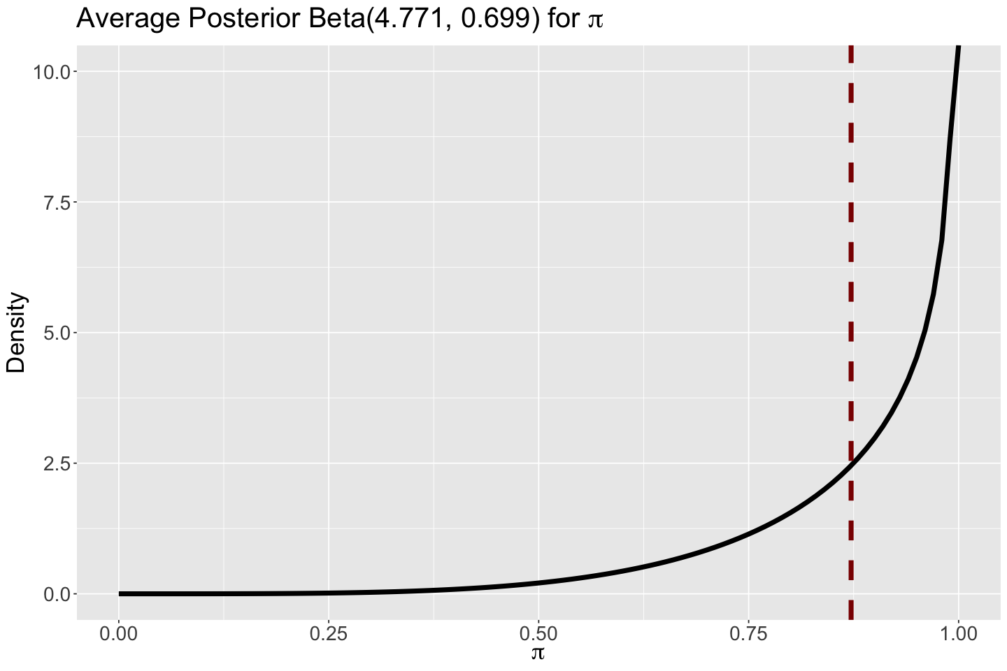
Then, using posterior means $a = 4.673$ and $b = 0.685$, we plot this average posterior theoretical Beta. Note that its corresponding mean $0.872$ is indicated as a vertical dashed line.

# Plotting average Beta posterior
average_beta_posterior <- ggplot() +
  xlim(0, 1) +
  ylim(0, 10) +
  geom_function(fun = dbeta, args = list(shape1 = 4.673, shape2 = 0.685), linewidth = 2) +
  geom_vline(xintercept = 0.872, colour = "darkred", linetype = "dashed", linewidth = 2) +
  theme(
    plot.title = element_text(size = 24),
    axis.text.x = element_text(size = 17, angle = 0),
    axis.text.y = element_text(size = 17, angle = 0),
    axis.title = element_text(size = 21),
  ) +
  labs(y = "Density", x = expression(pi)) +
  ggtitle(expression(paste("Average Posterior Beta(4.771, 0.699) for ", pi)))

This average Beta posterior leans more towards high probabilities for launch success given the evidence provided by all rockets along with our priors.

options(repr.plot.height = 8, repr.plot.width = 12)

average_beta_posterior

../_images/98aafc2edaea764c7fffe68c54a7e2b81e24bef8eb23e3b9a5e4f583ecc2f2ca.png

6.5. Prediction for a New Rocket#

We will modify our Hierarchical_Rocket model to incorporate the block generated quantities for a predicted probability pi_pred. We use the same process described in Lecture 5 - Bayesian Normal Linear Regression and Hypothesis Testing to obtain predictions. This process considers the posterior variability in parameters and the sampling variability. The predictive samples will yield a posterior predictive distribution for pi_pred.

pred_Hierarchical_Rocket <- "data {                          
int<lower=1> num_rockets;    // number of rockets 
int<lower=0> X[num_rockets];  // vector with sucesses by rocket
int<lower=1> n[num_rockets];  // vector with trials by rocket
}
parameters {
vector<lower=0,upper=1>[num_rockets] pi; // vector of 367 probabilities of launch success
real<lower=0> a; // beta parameter
real<lower=0> b; // beta parameter
}
model {
a ~ gamma(0.001, 0.001);     // prior for a
b ~ gamma(0.001, 0.001);     // prior for b

for (i in 1:num_rockets){
pi[i] ~ beta(a,b);           // modelling the pi_i by rocket
X[i] ~ binomial(n[i],pi[i]); // modelling the likelihood by rocket
}
}
generated quantities {
  real<lower=0,upper=1> pi_pred = beta_rng(a, b);
}"

The MCMC simulation uses the same Hierarchical_Rocket_dictionary but the modified pred_Hierarchical_Rocket.

pred_posterior_Hierarchical_Rocket <- stan(
  model_code = pred_Hierarchical_Rocket,
  data = Hierarchical_Rocket_dictionary,
  chains = 1,
  iter = 10000,
  warmup = 1000,
  thin = 5,
  seed = 553,
)

SAMPLING FOR MODEL 'anon_model' NOW (CHAIN 1).
Chain 1: 
Chain 1: Gradient evaluation took 8.4e-05 seconds
Chain 1: 1000 transitions using 10 leapfrog steps per transition would take 0.84 seconds.
Chain 1: Adjust your expectations accordingly!
Chain 1: 
Chain 1: 
Chain 1: Iteration:    1 / 10000 [  0%]  (Warmup)
Chain 1: Iteration: 1000 / 10000 [ 10%]  (Warmup)
Chain 1: Iteration: 1001 / 10000 [ 10%]  (Sampling)
Chain 1: Iteration: 2000 / 10000 [ 20%]  (Sampling)
Chain 1: Iteration: 3000 / 10000 [ 30%]  (Sampling)
Chain 1: Iteration: 4000 / 10000 [ 40%]  (Sampling)
Chain 1: Iteration: 5000 / 10000 [ 50%]  (Sampling)
Chain 1: Iteration: 6000 / 10000 [ 60%]  (Sampling)
Chain 1: Iteration: 7000 / 10000 [ 70%]  (Sampling)
Chain 1: Iteration: 8000 / 10000 [ 80%]  (Sampling)
Chain 1: Iteration: 9000 / 10000 [ 90%]  (Sampling)
Chain 1: Iteration: 10000 / 10000 [100%]  (Sampling)
Chain 1: 
Chain 1:  Elapsed Time: 1.792 seconds (Warm-up)
Chain 1:                12.019 seconds (Sampling)
Chain 1:                13.811 seconds (Total)
Chain 1: 

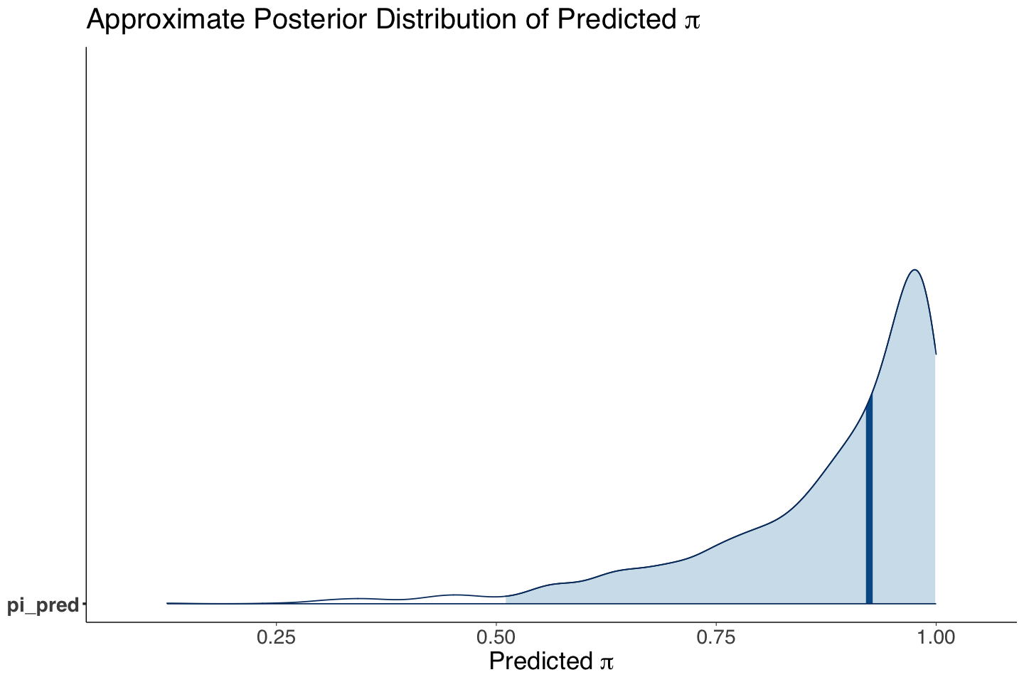
We only need the posterior metrics for pi_pred. Note the mean is extremely similar to the overall mean of $\pi$! Moreover, the posterior predictive distribution in post_hist_Hierarchical_Rocket_pi_pred is similar to average_beta_posterior.

summary_Hierarchical_Rocket_pi_pred <- as.data.frame(summary(pred_posterior_Hierarchical_Rocket)$summary)
summary_Hierarchical_Rocket_pi_pred <- summary_Hierarchical_Rocket_pi_pred[370, c("mean", "sd", "2.5%", "97.5%")] |>
  mutate_if(is.numeric, round, 3)
summary_Hierarchical_Rocket_pi_pred

A data.frame: 1 × 4
	mean	sd	2.5%	97.5%
	<dbl>	<dbl>	<dbl>	<dbl>
pi_pred	0.876	0.135	0.511	0.999

post_hist_Hierarchical_Rocket_pi_pred <- mcmc_areas(pred_posterior_Hierarchical_Rocket, pars = c("pi_pred"), prob = 0.95) +
  theme(
    plot.title = element_text(size = 24, family = "sans"),
    axis.text.x = element_text(size = 17, angle = 0, family = "sans"),
    axis.text.y = element_text(size = 17, angle = 0, family = "sans"),
    axis.title = element_text(size = 21, family = "sans"),
    strip.text.x = element_text(size = 21, family = "sans")
  ) +
  ggtitle(expression(paste("Approximate Posterior Distribution of Predicted ", pi))) +
  xlab(expression(paste("Predicted ", pi)))

post_hist_Hierarchical_Rocket_pi_pred

../_images/e1184385e28d1998d26eca48de8c3d21ed7a4ccf091456f8e6bd1498c0c33bab.png

Why do we have these similarities?

Our launch success mean posterior prediction for a new rocket is similar to the posterior mean of $\pi$ because this is the best Bayesian model we can obtain without further covariates (or features)! So, this is a mean probability prediction for the rocket population for a launch success.

7. Wrapping Up#

Even though hierarchical models involve more Bayesian complexity, they are helpful to take the best from non-pooled and pooled models.
These hierarchical models are also flexible enough to provide predictions for new observations.
We saw a model without covariates. Nevertheless, the hierarchical approach can be extended to Bayesian regression models. These are the counterpart of frequentist mixed-effects models.