Lecture 8 - More Hierarchical Modelling and MCMC Diagnostics

Lecture 8 - More Hierarchical Modelling and MCMC Diagnostics#

Today’s Learning Objectives#

Apply Bayesian hierarchical modelling in a more complex case.
Formulate the Bayesian modelling setup in this complex case.
Interpret the simulation results in function of the initial statistical inquiries.
Evaluate Markov Chain Monte Carlo (MCMC) posterior sampling via model diagnostics.

Loading `R` Packages#

options(repr.matrix.max.rows = 8)
library(bayesrules)
library(tidyverse)
library(rstan)
library(bayesplot)
library(cowplot)

1. The Spotify Dataset#

We will explore the spotify dataset from the bayesrules package. This dataset is a sample of $n = 350$ songs with different variables by column. The songs belong to 44 different artists. The package’s description is the following:

A sub-sample of the Spotify song data originally collected by Kaylin Pavlik (kaylinquest) and distributed through the R for Data Science TidyTuesday project.

If you like dancing, you might wonder: how danceable Spotify’s songs are?#

1.1. Main Statistical Inquiries#

Firstly, let us formally define our main statistical inquiries:

Assuming the spotify sample is representative enough, what is the overall mean danceability for the songs on the platform?
Assuming the spotify sample is representative enough of the 44 artists’ discography, how danceable is their music compared to the overall mean danceability of the songs in the platform?

Note

This exercise is based on Chapter 16 from Bayes Rules! textbook. However, they play around with a popularity index. Hence, let us make everything more danceable.

1.2. Data Wrangling#

The raw dataset has 23 columns, but our Bayesian model will be restricted to two of the them:

artist: song artist (a factor-type variable with 44 levels).
danceability: a continuous score from 0 (not danceable) to 100 (danceable) based on features such as tempo, rhythm, etc.

# Creating training set.
spotify_training <-spotify |>
  select(artist, danceability)
spotify_training

A tibble: 350 × 2
artist	danceability
<fct>	<dbl>
Alok	74.7
Alok	70.7
Alok	77.8
Alok	68.2
⋮	⋮
Zeds Dead	65.9
Zeds Dead	60.4
Zeds Dead	50.1
Zeds Dead	67.5

As in the baseball problem from lab2, we will have an ID catalogue for artists. Hence, we create a catalogue of artist names and assign numerical codes from 1 to 44 by alphabetical order. We will use this catalogue in our Bayesian results later on.

artist_catalogue <- tibble(
  artist = levels(spotify_training$artist),
  code = 1:44
)

1.3. Exploratory Data Analysis#

Let us make a quick exploratory data analysis (EDA) via side-by-side boxplots for artist versus danceability.

options(repr.plot.height = 8, repr.plot.width = 12)

danceability_boxplots <- spotify_training |>
  ggplot(aes(reorder(artist, danceability), danceability)) +
  geom_boxplot(aes(fill = artist)) +
  labs(y = "Danceability Score", x = "Artist") +
  ggtitle("Side-by-Side Boxplots") +
  theme(
    plot.title = element_text(size = 24, face = "bold"),
    axis.text = element_text(size = 17, angle = 90),
    axis.title = element_text(size = 21),
    legend.position = "none"
  )

danceability_boxplots

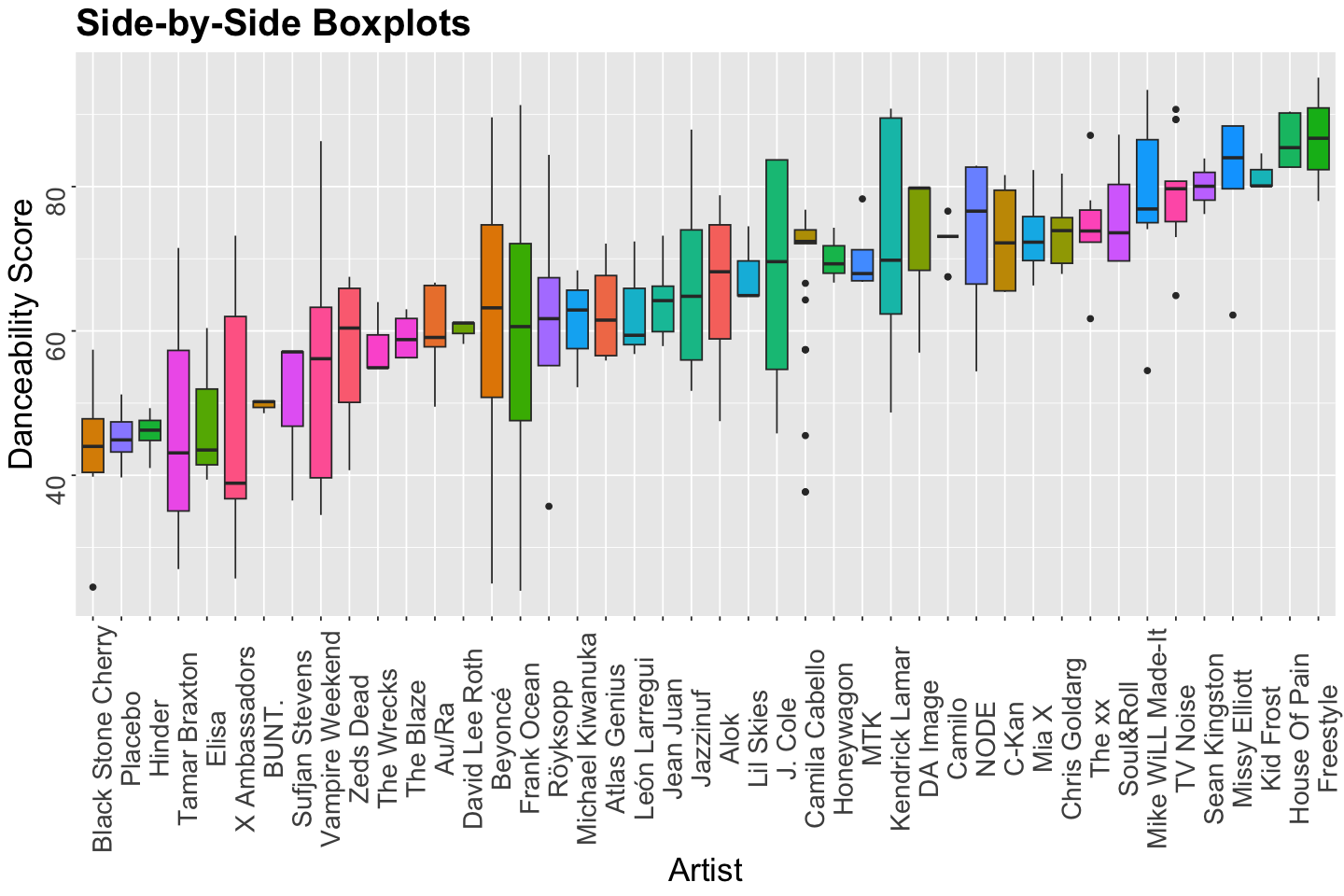
../_images/b3f9f2ad9b6750987b430d9b822ba2f7a79eaeafb6bc3ec53f026ae938c48dc8.png

The EDA gives us graphical insights into what artists are the most danceable. Nonetheless, this is only a sample! We need to set up a proper inferential model for our population of interest.

Moreover, keep in mind the variability from artist to artist. Our Bayesian model needs to take this matter into account.

2. The Bayesian Hierarchical Model#

According to our main statistical inquiries, let us start with hierarchical modelling.

2.1. The Likelihood#

Let $Y_{i,j}$ be danceability score for the $i$th song in spotify_training (i.e., a row $i = 1, \dots, 350$) for the $j$th artist (a level in artist $j = 1, \dots, 44$). We will use a Normal likelihood:

\[Y_{i,j} \mid \mu_j, \sigma_w \sim \mathcal{N}(\mu_j, \sigma^2_w);\]

where $\mu_j$ is the mean danceability score for the $j$th artist and $\sigma_w$ is the standard deviation representing the within-artist variability IN GENERAL. Their observations correspond to songs.

Exercise 23

Since danceability is bounded between 0 and 100, what other ideal distribution can we use aside from an unbounded Normal likelihood?

A. A Negative Binomial distribution.

B. A Gamma distribution.

C. A Beta distribution.

D. A Poisson distribution.

How can we set up the overall mean $\mu$?

This can be done by decomposing the mean $\mu_j$ for the $j$th artist as follows:

\[\mu_j = \mu + b_j;\]

where $\mu$ is the overall mean danceability for all the songs in the platform (i.e., our first inquiry!), and $b_j$ is the mean danceability deviation of the $j$th artist to the overall mean $\mu$ (i.e., our second inquiry!). Note we will have 44 different $b_j$s since we have 44 artists. Furthermore, these deviations can be either positive or negative.

So far we have these parameters of interest:

Overall mean danceability $\mu$.
44 mean danceability devations $b_j$.
Within-group (i.e., within artist) variability via the standard deviation $\sigma_w$.

2.2. The Priors#

Now, let us set the priors as a hierarchical model. For our 44 deviations $b_j$, we will have:

\[b_j \mid \sigma_\mu \sim \mathcal{N}(0, \sigma_\mu^2);\]

we assume a mean zero since we do not know whether the $j$th artist danceability will differ in average from the overall mean danceability $\mu$.

Note we have another parameter of interest: the between-artist variability represented by the standard deviation $\sigma_\mu$. Therefore, we are basically decomposing the variance for the $i$th song and $j$th artist as:

\[\text{Var}\big(Y_{i,j}\big) = \sigma_\mu^2 + \sigma^2_w.\]

Here comes the hierarchical twist…

The between-artist variability represented by the standard deviation $\sigma_\mu$ will also have a prior. We are doing this to make our model flexible enough to apply the “borrowing strength” idea. Hence, the prior will be an Exponential distribution (non-negative continuous) since $\sigma_\mu$ is a standard deviation:

\[\sigma_\mu \sim \text{Exponential}(0.048),\]

which assigns higher probabilities to large values (i.e, we believe there is a huge variability in danceability between artists in our prior).

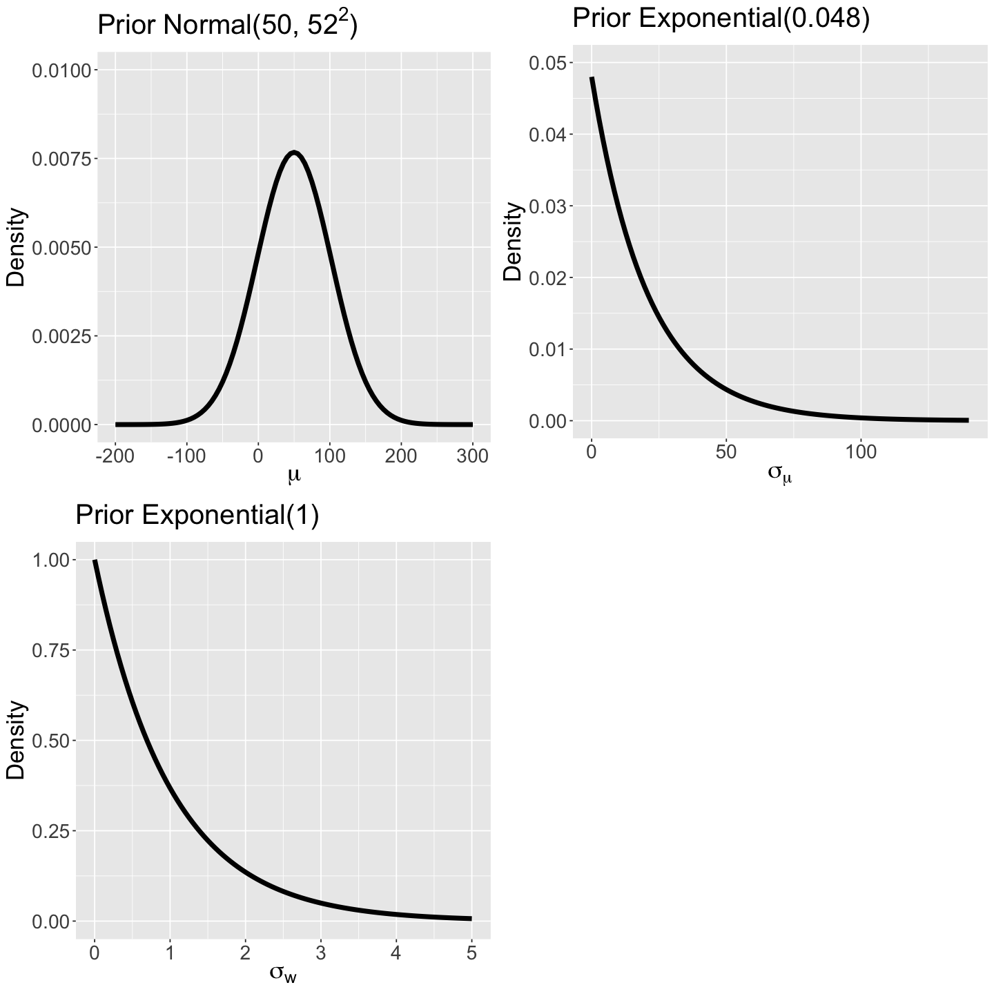
Finally, we need to set up priors for the overall mean danceability $\mu$ and within-artist variability via the standard deviation $\sigma_w$:

\[\mu \sim \mathcal{N}(50, 52^2)\]

\[\sigma_w \sim \text{Exponential}(1).\]

The prior for the overall mean danceability $\mu$ assigns a middle ground with high variability, while $\sigma_w$ has a prior assigning higher probabilities to values between 0 and 2. (compared to the prior of $\sigma_{\mu}$). This prior belief denotes a moderate variability in danceability in the artist’s catalogue.

prior_normal_50_52 <- ggplot() +
  xlim(-200, 300) +
  ylim(0, 0.01) +
  geom_function(fun = dnorm, args = list(mean = 50, sd = 52), linewidth = 2) +
  theme(
    plot.title = element_text(size = 24),
    axis.text.x = element_text(size = 17, angle = 0),
    axis.text.y = element_text(size = 17, angle = 0),
    axis.title = element_text(size = 21),
  ) +
  labs(y = "Density", x = expression(mu)) +
  ggtitle(expression(paste("Prior Normal(50, ", 52^2, ")")))

prior_exp_0.048 <- ggplot() +
  xlim(0, 140) +
  ylim(0, 0.05) +
  geom_function(fun = dexp, args = list(rate = 0.048), linewidth = 2) +
  theme(
    plot.title = element_text(size = 24),
    axis.text.x = element_text(size = 17, angle = 0),
    axis.text.y = element_text(size = 17, angle = 0),
    axis.title = element_text(size = 21),
  ) +
  labs(y = "Density", x = expression(sigma[mu])) +
  ggtitle(expression("Prior Exponential(0.048)"))

prior_exp_1 <- ggplot() +
  xlim(0, 5) +
  ylim(0, 1) +
  geom_function(fun = dexp, args = list(rate = 1), linewidth = 2) +
  theme(
    plot.title = element_text(size = 24),
    axis.text.x = element_text(size = 17, angle = 0),
    axis.text.y = element_text(size = 17, angle = 0),
    axis.title = element_text(size = 21),
  ) +
  labs(y = "Density", x = expression(sigma["w"])) +
  ggtitle(expression("Prior Exponential(1)"))

options(repr.plot.height = 12, repr.plot.width = 12)

plot_grid(prior_normal_50_52, prior_exp_0.048, prior_exp_1)

../_images/29be9e5a4eac816e55914e455be2e37d3ac119892e6896f1cdfb9d448ae10fb9.png

The formal Bayesian hierarchical model is set up as:

\[\begin{split}\begin{align*} \text{likelihood:} \qquad Y_{i,j} \mid \mu_j, \sigma_w \sim \mathcal{N}(\mu_j, \sigma^2_w) \\ \text{where} \quad \mu_j = \mu + b_j \\ \text{priors:} \quad b_j \mid \sigma_\mu \sim \mathcal{N}(0, \sigma_\mu^2) \\ \qquad \mu \sim \mathcal{N}(50, 52^2) \\ \qquad \sigma_w \sim \text{Exponential}(1) \\ \qquad \sigma_\mu \sim \text{Exponential}(0.048). \end{align*}\end{split}\]

Exercise 24

What other prior distribution can we use for both types of variance?

A. A Gamma distribution.

B. A Binomial distribution.

C. A Poisson distribution.

D. A Chi-squared distribution.

2.3. Coding the Model#

We code up this spotify_model model on Stan. The structure is similar to the baseball case from lab2.

spotify_model <- "data {                          
int<lower=1> n;                     //rows in training set
int<lower=1> num_artist;            //number of artists in training set
int<lower=1> artist[n];             //artist ID column by song in training set
vector[n] dance_score;              //danceability scores by song in training set             
}
parameters {
vector[num_artist] mean_dance;      //vector of posterior danceability score deviations for each artist (size num_artist)
real overall_mean;                  //overall mean in danceability score
real<lower=0> between_sigma;        //between-artist sd in danceability score
real<lower=0> within_sigma;         //within-artist sd in danceability score
}
model {
between_sigma ~ exponential(0.048);     //between-artist sd prior
within_sigma ~ exponential(1);  //within-artist sd prior
overall_mean ~ normal(50, 52);      //overall mean prior
for (j in 1:num_artist){            //danceability scores priors (deviations per artist)
  mean_dance[j] ~ normal(0, between_sigma);
}
for (i in 1:n){
  int artist_index = artist[i];     //auxiliary indexing variable
  dance_score[i] ~ normal(overall_mean + mean_dance[artist_index], within_sigma); //likelihood in training set
}
}"

2.4. Running the MCMC Simulation#

Before creating the spotify_dictionary, we switch the ID names to numerical codes from 1 to 44 according to the alphabetical order in the levels of spotify_training$artist. We need to do this since we cannot work with factor levels in Stan. Then, we run the simulation.

levels(spotify_training$artist) <- 1:44

spotify_dictionary <- list(
  n = nrow(spotify_training),
  num_artist = nrow(artist_catalogue),
  artist = as.integer(spotify_training$artist),
  dance_score = spotify_training$danceability
)

posterior_spotify <- stan(
  model_code = spotify_model,
  data = spotify_dictionary,
  chains = 1,
  iter = 20000,
  warmup = 2000,
  thin = 20,
  seed = 553
)

SAMPLING FOR MODEL 'anon_model' NOW (CHAIN 1).
Chain 1: 
Chain 1: Gradient evaluation took 5.9e-05 seconds
Chain 1: 1000 transitions using 10 leapfrog steps per transition would take 0.59 seconds.
Chain 1: Adjust your expectations accordingly!
Chain 1: 
Chain 1: 
Chain 1: Iteration:     1 / 20000 [  0%]  (Warmup)
Chain 1: Iteration:  2000 / 20000 [ 10%]  (Warmup)
Chain 1: Iteration:  2001 / 20000 [ 10%]  (Sampling)
Chain 1: Iteration:  4000 / 20000 [ 20%]  (Sampling)
Chain 1: Iteration:  6000 / 20000 [ 30%]  (Sampling)
Chain 1: Iteration:  8000 / 20000 [ 40%]  (Sampling)
Chain 1: Iteration: 10000 / 20000 [ 50%]  (Sampling)
Chain 1: Iteration: 12000 / 20000 [ 60%]  (Sampling)
Chain 1: Iteration: 14000 / 20000 [ 70%]  (Sampling)
Chain 1: Iteration: 16000 / 20000 [ 80%]  (Sampling)
Chain 1: Iteration: 18000 / 20000 [ 90%]  (Sampling)
Chain 1: Iteration: 20000 / 20000 [100%]  (Sampling)
Chain 1: 
Chain 1:  Elapsed Time: 1.409 seconds (Warm-up)
Chain 1:                6.71 seconds (Sampling)
Chain 1:                8.119 seconds (Total)
Chain 1: 

2.5. Output Summary#

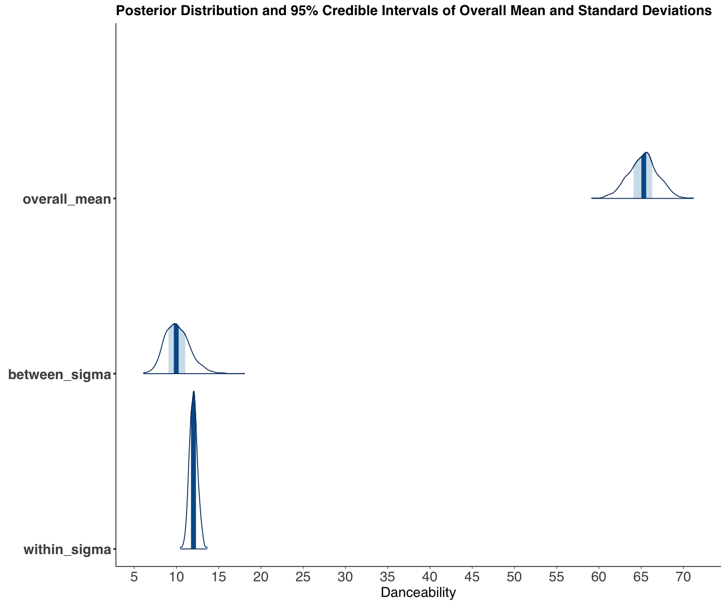
We obtain the output from posterior_spotify. Firstly, let us focus the attention on the overall danceability $\mu$ (overall_mean), the between-artist standard deviation $\sigma_\mu$ (between_sigma), and within-artist standard deviation $\sigma_w$ (within_sigma).

summary_overall <- as.data.frame(summary(posterior_spotify)$summary)
summary_overall <- summary_overall[45:47, c("mean", "sd", "2.5%", "97.5%")] |>
  mutate_if(is.numeric, round, 3)
summary_overall

A data.frame: 3 × 4
	mean	sd	2.5%	97.5%
	<dbl>	<dbl>	<dbl>	<dbl>
overall_mean	65.228	1.751	61.744	68.579
between_sigma	10.128	1.504	7.588	13.373
within_sigma	12.013	0.476	11.126	12.984

For our first inquiry, we can conclude the following:

The overall danceability $\mu$ is between 61.744 and 68.579 with 95% probability and a posterior mean of 65.228.
Moreover, we see more variability associated with the between-artist standard deviation $\sigma_\mu$ which makes sense (artist diversity should be large in the platform!). Note the 95% credible interval between 7.588 and 13.373.
On the other hand, the within-artist variability $\sigma_w$ shows less variability. Note the 95% credible interval between 11.126 and 12.984.

options(repr.plot.height = 10, repr.plot.width = 12)

post_hist_spotify <- mcmc_areas(posterior_spotify, pars = c(
  "overall_mean",
  "between_sigma",
  "within_sigma"
)) +
  theme(
    plot.title = element_text(size = 16.5, face = "bold", family = "sans"),
    axis.text.x = element_text(size = 16.5, angle = 0, family = "sans"),
    axis.text.y = element_text(size = 16.5, angle = 0, family = "sans"),
    axis.title = element_text(size = 16.5, family = "sans"),
    strip.text.x = element_text(size = 16.5, family = "sans")
  ) +
  ggtitle("Posterior Distribution and 95% Credible Intervals of Overall Mean and Standard Deviations") +
  scale_x_continuous(breaks = seq(0, 70, 5)) +
  xlab("Danceability")

Scale for x is already present.
Adding another scale for x, which will replace the existing scale.

post_hist_spotify

../_images/8fd135102d4b25eee8372270038787c3ea0f9717cd95c08abb7b49f7fc6ceda0.png

What about the mean danceability deviations by artist $b_j$?

Recall these deviations could be positive or negative given how we modelled them:

\[\mu_j = \mu + b_j.\]

Since Stan labels the parameters in the posterior samples as mean_dance[1], …, mean_dance[44], we will add a new column with the actual artist name stored in artist_catalogue.

summary_artist_means <- as.data.frame(summary(posterior_spotify)$summary)
summary_artist_means <- summary_artist_means[1:44, c("mean", "sd", "2.5%", "97.5%")] |>
  mutate_if(is.numeric, round, 3)
summary_artist_means$artist <- as.factor(artist_catalogue$artist)
summary_artist_means |>
  arrange(-mean) 

A data.frame: 44 × 5
	mean	sd	2.5%	97.5%	artist
	<dbl>	<dbl>	<dbl>	<dbl>	<fct>
mean_dance[18]	16.324	5.072	6.793	26.317	House Of Pain
mean_dance[15]	14.339	5.997	3.167	27.308	Freestyle
mean_dance[41]	12.673	3.437	5.771	19.364	TV Noise
mean_dance[29]	11.903	4.897	2.387	21.454	Missy Elliott
⋮	⋮	⋮	⋮	⋮	⋮
mean_dance[43]	-14.321	4.350	-22.955	-6.364	X Ambassadors
mean_dance[16]	-15.724	4.758	-25.361	-6.106	Hinder
mean_dance[32]	-16.089	4.691	-25.402	-7.092	Placebo
mean_dance[5]	-17.585	4.517	-26.706	-9.478	Black Stone Cherry

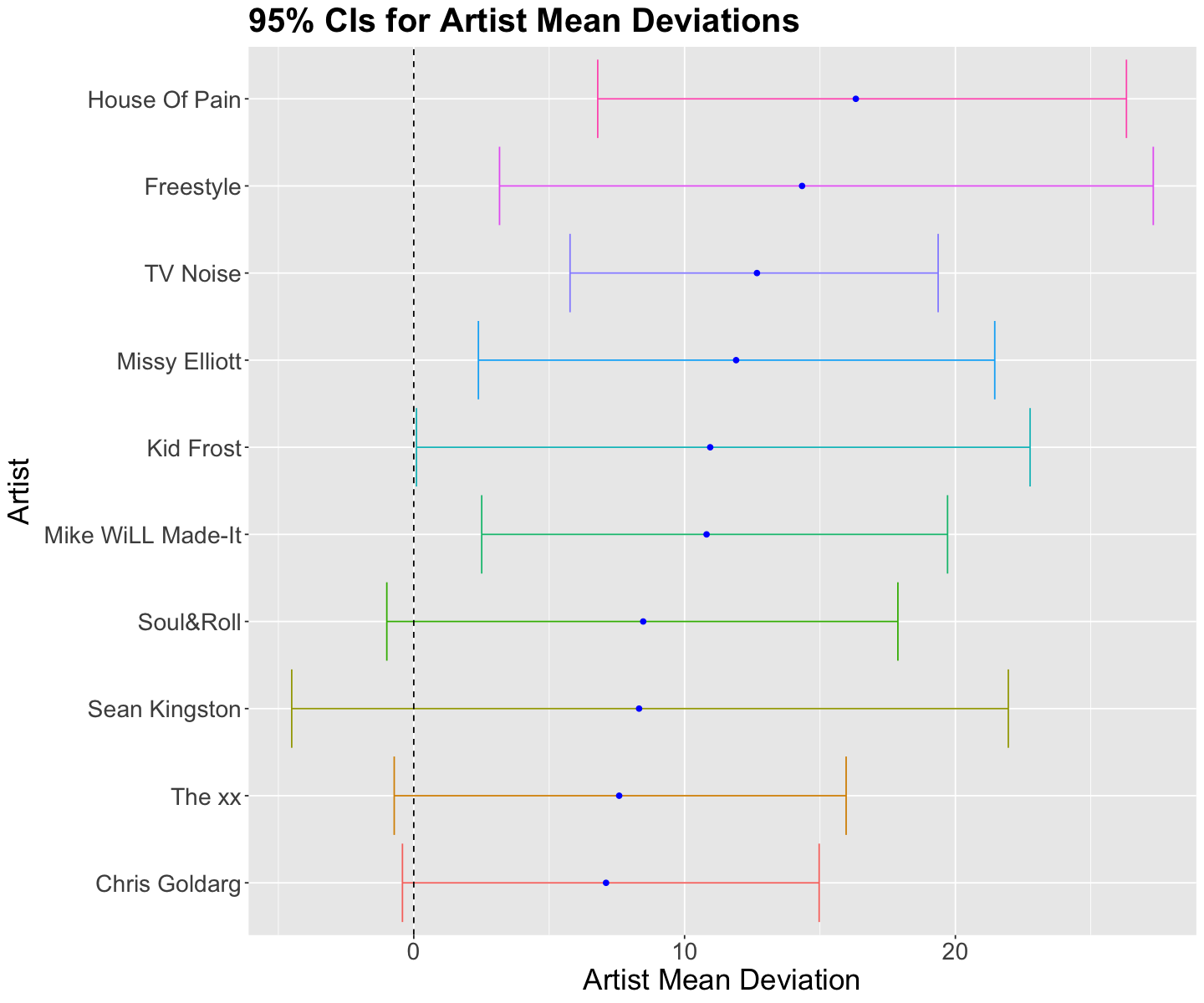
Recall our second inquiry:

Assuming the spotify dataset is representative enough of the 44 artists discography, how danceable is their music compared to the overall mean danceability for the songs on the platform?

Let us focus on the top 10 posterior means for deviation $b_j$ (they are plotted below along with their 95% credible intervals). Four artists have their credible intervals with positive bounds (i.e., there is a 95% probability they are more danceable than the overall danceability mean $\mu$!): House of Pain, Freestyle, TV Noise, and Missy Elliot.

posterior_artist_means_CIs_plot <- summary_artist_means |>
  arrange(-mean) |>
  slice(1:10) |>
  mutate(artist = fct_reorder(artist, mean)) |>
  ggplot(aes(x = mean, y = artist)) +
  geom_errorbarh(aes(xmax = `2.5%`, xmin = `97.5%`, color = artist)) +
  geom_point(color = "blue") +
  theme(
    plot.title = element_text(size = 24, face = "bold"),
    axis.text = element_text(size = 17),
    axis.title = element_text(size = 21),
    legend.position = "none"
  ) +
  ggtitle("95% CIs for Artist Mean Deviations") +
  labs(x = "Artist Mean Deviation", y = "Artist") +
  geom_vline(xintercept = 0, linetype = "dashed")

posterior_artist_means_CIs_plot

../_images/c4a9bca5e149a1c3bca143e24c9492e02ff7e3ffeda3fade7494cc8c4a8f7e0b.png

Even though the hierarchical model can reduce the variability in our posterior estimates, we need to help it by including features! Since

\[\mu_j = \mu + b_j,\]

we might break down the mean deviation $b_j$ with a regression systematic component. This is a potential improvement for this model!

3. MCMC Diagnostics#

This is the last topic of the block, and it will allow evaluating the MCMC posterior sampling quality.

There are many potential pitfalls in MCMC: not enough iterations, not enough thinning, not enough burn-in, etc. So how do we know if it worked and is giving us “good” samples from the approximate posterior distribution? Thankfully, there are MCMC convergence diagnostics to provide us with a sense of whether we can trust the output of our MCMC algorithm.

We are sampling via a Markov chain; thus, our sampled elements (i.e., “links” in the chain) will not be fully independent. However, we can make them “semi-independent” with the thin argument. Nonetheless, each Bayesian case behaves differently, and some are harder than others. Therefore, thinning can sometimes be less effective.

Furthermore, a common practice is to sample via more than one chain. We would expect sampling consistency across all chains.

Warning

Sampling consistency across chains does not necessarily implicate the algorithm walks are quickly converging in all chains. That said, all sampling chains could also be equally bad!

To illustrate the use of MCMC diagnostics, let us sample four chains for the previous Spotify case. We will have the following number of posterior samples by chain:

\[\texttt{samples} = \frac{\texttt{iterations} - \texttt{warmup}}{\texttt{thin}} = \frac{20,000 - 2,000}{20} = 900.\]

posterior_spotify_4_chains <- stan(
  model_code = spotify_model,
  data = spotify_dictionary,
  chains = 4,
  iter = 20000,
  warmup = 2000,
  thin = 20,
  seed = 553
)

SAMPLING FOR MODEL 'anon_model' NOW (CHAIN 1).
Chain 1: 
Chain 1: Gradient evaluation took 2.3e-05 seconds
Chain 1: 1000 transitions using 10 leapfrog steps per transition would take 0.23 seconds.
Chain 1: Adjust your expectations accordingly!
Chain 1: 
Chain 1: 
Chain 1: Iteration:     1 / 20000 [  0%]  (Warmup)
Chain 1: Iteration:  2000 / 20000 [ 10%]  (Warmup)
Chain 1: Iteration:  2001 / 20000 [ 10%]  (Sampling)
Chain 1: Iteration:  4000 / 20000 [ 20%]  (Sampling)
Chain 1: Iteration:  6000 / 20000 [ 30%]  (Sampling)
Chain 1: Iteration:  8000 / 20000 [ 40%]  (Sampling)
Chain 1: Iteration: 10000 / 20000 [ 50%]  (Sampling)
Chain 1: Iteration: 12000 / 20000 [ 60%]  (Sampling)
Chain 1: Iteration: 14000 / 20000 [ 70%]  (Sampling)
Chain 1: Iteration: 16000 / 20000 [ 80%]  (Sampling)
Chain 1: Iteration: 18000 / 20000 [ 90%]  (Sampling)
Chain 1: Iteration: 20000 / 20000 [100%]  (Sampling)
Chain 1: 
Chain 1:  Elapsed Time: 1.294 seconds (Warm-up)
Chain 1:                5.628 seconds (Sampling)
Chain 1:                6.922 seconds (Total)
Chain 1: 

SAMPLING FOR MODEL 'anon_model' NOW (CHAIN 2).
Chain 2: 
Chain 2: Gradient evaluation took 2e-05 seconds
Chain 2: 1000 transitions using 10 leapfrog steps per transition would take 0.2 seconds.
Chain 2: Adjust your expectations accordingly!
Chain 2: 
Chain 2: 
Chain 2: Iteration:     1 / 20000 [  0%]  (Warmup)
Chain 2: Iteration:  2000 / 20000 [ 10%]  (Warmup)
Chain 2: Iteration:  2001 / 20000 [ 10%]  (Sampling)
Chain 2: Iteration:  4000 / 20000 [ 20%]  (Sampling)
Chain 2: Iteration:  6000 / 20000 [ 30%]  (Sampling)
Chain 2: Iteration:  8000 / 20000 [ 40%]  (Sampling)
Chain 2: Iteration: 10000 / 20000 [ 50%]  (Sampling)
Chain 2: Iteration: 12000 / 20000 [ 60%]  (Sampling)
Chain 2: Iteration: 14000 / 20000 [ 70%]  (Sampling)
Chain 2: Iteration: 16000 / 20000 [ 80%]  (Sampling)
Chain 2: Iteration: 18000 / 20000 [ 90%]  (Sampling)
Chain 2: Iteration: 20000 / 20000 [100%]  (Sampling)
Chain 2: 
Chain 2:  Elapsed Time: 1.411 seconds (Warm-up)
Chain 2:                6.336 seconds (Sampling)
Chain 2:                7.747 seconds (Total)
Chain 2: 

SAMPLING FOR MODEL 'anon_model' NOW (CHAIN 3).
Chain 3: 
Chain 3: Gradient evaluation took 2.2e-05 seconds
Chain 3: 1000 transitions using 10 leapfrog steps per transition would take 0.22 seconds.
Chain 3: Adjust your expectations accordingly!
Chain 3: 
Chain 3: 
Chain 3: Iteration:     1 / 20000 [  0%]  (Warmup)
Chain 3: Iteration:  2000 / 20000 [ 10%]  (Warmup)
Chain 3: Iteration:  2001 / 20000 [ 10%]  (Sampling)
Chain 3: Iteration:  4000 / 20000 [ 20%]  (Sampling)
Chain 3: Iteration:  6000 / 20000 [ 30%]  (Sampling)
Chain 3: Iteration:  8000 / 20000 [ 40%]  (Sampling)
Chain 3: Iteration: 10000 / 20000 [ 50%]  (Sampling)
Chain 3: Iteration: 12000 / 20000 [ 60%]  (Sampling)
Chain 3: Iteration: 14000 / 20000 [ 70%]  (Sampling)
Chain 3: Iteration: 16000 / 20000 [ 80%]  (Sampling)
Chain 3: Iteration: 18000 / 20000 [ 90%]  (Sampling)
Chain 3: Iteration: 20000 / 20000 [100%]  (Sampling)
Chain 3: 
Chain 3:  Elapsed Time: 1.52 seconds (Warm-up)
Chain 3:                6.323 seconds (Sampling)
Chain 3:                7.843 seconds (Total)
Chain 3: 

SAMPLING FOR MODEL 'anon_model' NOW (CHAIN 4).
Chain 4: 
Chain 4: Gradient evaluation took 2.2e-05 seconds
Chain 4: 1000 transitions using 10 leapfrog steps per transition would take 0.22 seconds.
Chain 4: Adjust your expectations accordingly!
Chain 4: 
Chain 4: 
Chain 4: Iteration:     1 / 20000 [  0%]  (Warmup)
Chain 4: Iteration:  2000 / 20000 [ 10%]  (Warmup)
Chain 4: Iteration:  2001 / 20000 [ 10%]  (Sampling)
Chain 4: Iteration:  4000 / 20000 [ 20%]  (Sampling)
Chain 4: Iteration:  6000 / 20000 [ 30%]  (Sampling)
Chain 4: Iteration:  8000 / 20000 [ 40%]  (Sampling)
Chain 4: Iteration: 10000 / 20000 [ 50%]  (Sampling)
Chain 4: Iteration: 12000 / 20000 [ 60%]  (Sampling)
Chain 4: Iteration: 14000 / 20000 [ 70%]  (Sampling)
Chain 4: Iteration: 16000 / 20000 [ 80%]  (Sampling)
Chain 4: Iteration: 18000 / 20000 [ 90%]  (Sampling)
Chain 4: Iteration: 20000 / 20000 [100%]  (Sampling)
Chain 4: 
Chain 4:  Elapsed Time: 1.812 seconds (Warm-up)
Chain 4:                6.322 seconds (Sampling)
Chain 4:                8.134 seconds (Total)
Chain 4: 

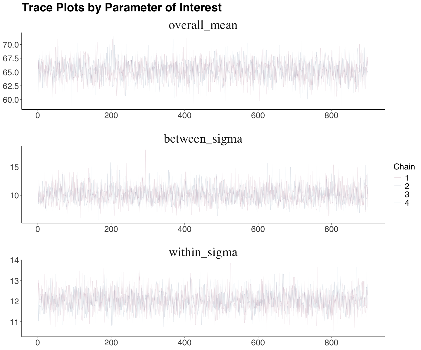
3.1. Trace Plots#

Trace plots horizontally illustrate the posterior sampling by a chain. All chain evolutions (excluding warmup) are overlaid. We will have a trace plot by a parameter of interest (here, we are only plotting overall_mean, between_sigma, and within_sigma for practical purposes).

Ideally, there should be a flat pattern by parameter without any upward or a downward trend throughout the chain. Moreover, we should not see any chain stuck. The function mcmc_trace() from bayesplot automatically displays these plots.

color_scheme_set("mix-blue-pink")

trace_spotify_4_chains <- mcmc_trace(posterior_spotify_4_chains,
  pars = c(
    "overall_mean",
    "between_sigma",
    "within_sigma"
  ),
  size = 0.1,
  facet_args = list(nrow = 3)
) +
  ggtitle("Trace Plots by Parameter of Interest") +
  theme(
    plot.title = element_text(size = 24, face = "bold", family = "sans"),
    axis.text = element_text(size = 17, family = "sans"),
    axis.title = element_text(size = 21, family = "sans"),
    legend.text = element_text(size = 17, family = "sans"),
    legend.title = element_text(size = 17, family = "sans")
  ) +
  facet_text(size = 26)

In the Spotify case (for overall_mean, between_sigma, and within_sigma), we see acceptable proper plots (flat horizontal trends and no chain stucks).

trace_spotify_4_chains

../_images/9661ffc5ffb48e1315e09968b557bcbfb5059e337fa1f576c16ef392d7d61ef2.png

The cases below belong to other toy examples (Beta-Binomial models) with bad MCMC samplings. Note the downward trend in Chain A and the sampling stuck in Chain B. The downward trend implicates the algorithm is sampling smaller parameter values throughout the simulation.

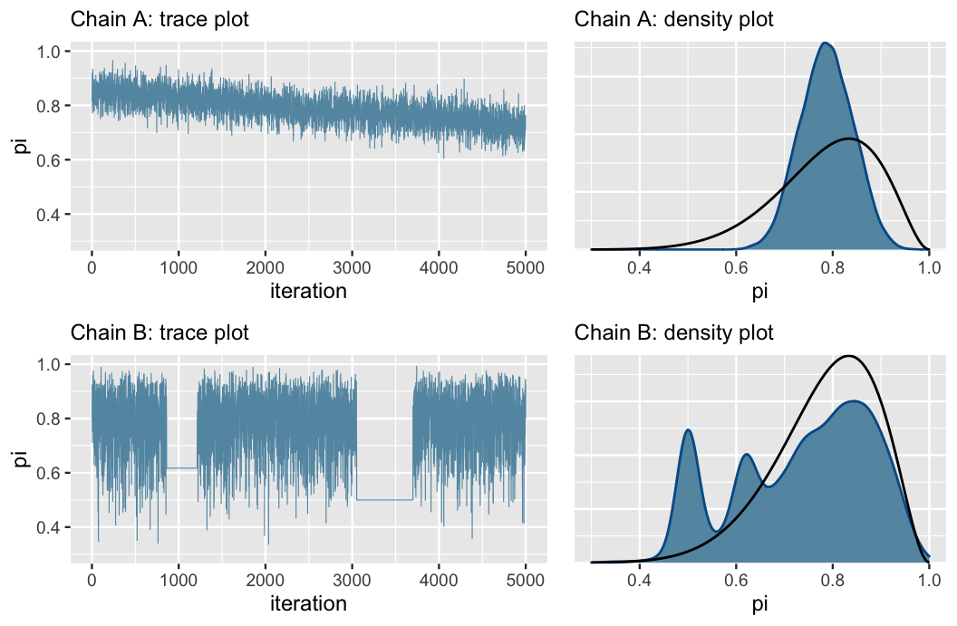
Source: Johnson et al. (2021)

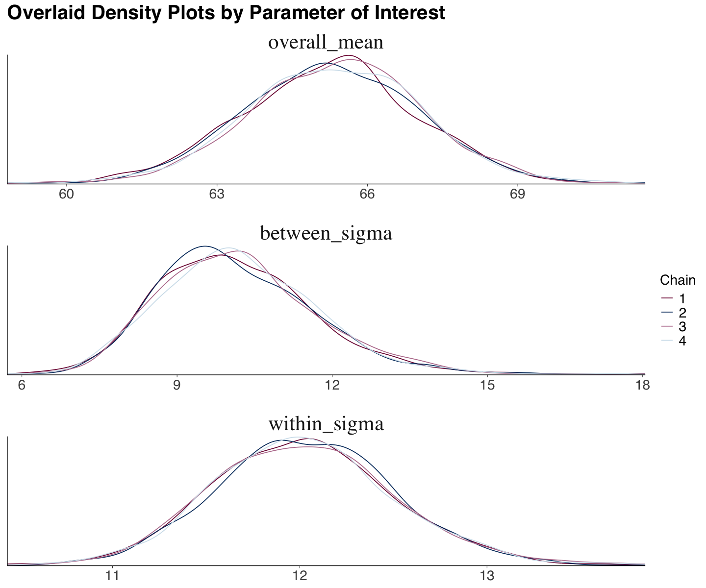
3.2. Empirical Density Plots#

We can also obtain empirical density plots for the parameters of interest with our MCMC posterior samples. The function mcmc_dens_overlay() from bayesplot automatically displays these overlaid plots (one by chain and parameter). Ideally, the overlaid plots would show similar behaviours to conclude chain consistency.

density_spotify_4_chains <- mcmc_dens_overlay(posterior_spotify_4_chains,
  pars = c(
    "overall_mean",
    "between_sigma",
    "within_sigma"),
  facet_args = list(nrow = 3)) +
  ggtitle("Overlaid Density Plots by Parameter of Interest") +
  theme(
    plot.title = element_text(size = 24, face = "bold", family = "sans"),
    axis.text = element_text(size = 17, family = "sans"),
    axis.title = element_text(size = 21, family = "sans"),
    legend.text = element_text(size = 17, family = "sans"),
    legend.title = element_text(size = 17, family = "sans")
  ) +
  facet_text(size = 26)

We see the same overall pattern with minor local variations in the Spotify case (for overall_mean, between_sigma, and within_sigma).

density_spotify_4_chains

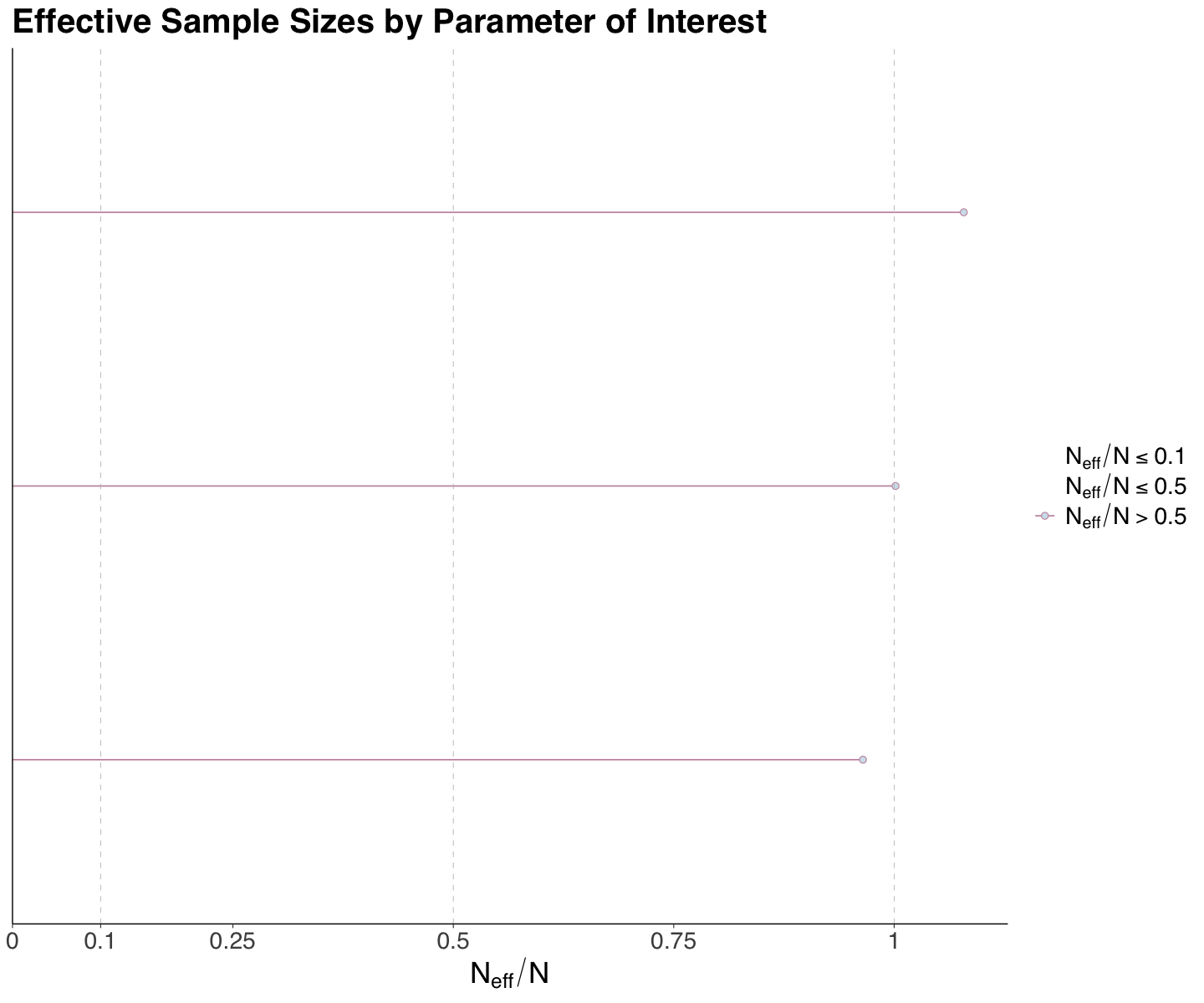
../_images/5682d2bf80b76ba0971b3d1e16487fb37d6a9f6bd93f5c31abcb41221fbc974b.png

3.3. Effective Sample Size#

The effective sample size $N_{\text{eff}}$ is a metric that measures the number of independent samples it would take to achieve an accurate MCMC posterior approximation.

If $N$ is the length of a given chain, given the characteristics of MCMC, we would expect that $N_{\text{eff}} < N$. Ideally, $N_{\text{eff}}$ should be as close as possible to $N$ or their correspoding ratio close to 1:

\[\frac{N_{\text{eff}}}{N}.\]

Important

Ideally, the above ratio should be as close as $1$ since $N_{\text{eff}}$ represents the number of fully independent posterior samples we would need to get an accurate posterior approximation (such as in a Monte Carlo simulation!). On the other hand, in practice, given its link structure and our warmup and thinning settings, MCMC would need more than $N_{\text{eff}}$ to achieve an accurate posterior approximation (i.e., $N > N_{\text{eff}}$). Nevertheless, it might be the case (as in this example) that this ratio can be larger than $1$ for standalone parameters.

Having said that, note we could have the following possible scenarios:

For a given standalone parameter, a ratio $\frac{N_{\text{eff}}}{N} < 1$ indicates that our MCMC sampling would need a larger number of samples $N$ to be as good as a Monte Carlo simulation. Again, recall we draw this conclusion per standalone parameter. Therefore, we would increase the number of iterations AND/OR thinning in the MCMC sampling once we see a big picture across all our parameters of interest in the model.
For a given standalone parameter, a ratio $\frac{N_{\text{eff}}}{N} = 1$ indicates that our MCMC sampling is as good as a Monte Carlo simulation. Again, recall we can only draw this conclusion per standalone parameter. If all the parameters of interest show ratios $\frac{N_{\text{eff}}}{N}$ close enough to $1$ (either slightly above or below), we could leave the sampling() setup as is. On the other hand, some parameters in the model will show a ratio close to $1$, while others will not. Thus, we might need to modify accordingly the number of iterations AND/OR thinning once we see a big picture across all our parameters of interest in the model.
For a given standalone parameter, a ratio $\frac{N_{\text{eff}}}{N} > 1$ indicates that our MCMC sampling needs less posterior samples $N$ to be as good as a Monte Carlo simulation. Again, recall we can only draw this conclusion per standalone parameter. Possibly, some parameters will show a ratio $> 1$ while others will have a ratio quite close or equal to $1$ (or even have a ratio $< 1$!). Thus, we might need to modify accordingly the number of iterations AND/OR thinning once we see a big picture across all our parameters of interest in the model.

The ratios, by parameter of interest, can be obtained via neff_ratio() from bayesplot. The specific mathematical computation for $N_{\text{eff}}$ can be found here.

spotify_eff_sample_size <- neff_ratio(posterior_spotify_4_chains,
  pars = c(
    "overall_mean",
    "between_sigma",
    "within_sigma")
)
round(spotify_eff_sample_size, 3)

overall_mean: 1.001
between_sigma: 1.079
within_sigma: 0.965

Our effective sample sizes for overall_mean, between_sigma, and within_sigma indicate an acceptable performance effective sample size (all three are around $1$).

We can use mcmc_neff() if we want to plot these ratios. For the Spotify case, there are no major concerns regarding these metrics.

eff_sample_size_4_chains <- mcmc_neff(spotify_eff_sample_size, size = 2) +
  ggtitle("Effective Sample Sizes by Parameter of Interest") +
  theme(
    plot.title = element_text(size = 24, face = "bold", family = "sans"),
    axis.text = element_text(size = 17, family = "sans"),
    axis.title = element_text(size = 21, family = "sans"),
    legend.text = element_text(size = 17, family = "sans"),
    legend.title = element_text(size = 17, family = "sans")
  ) +
  facet_text(size = 26)

eff_sample_size_4_chains

../_images/32fead138ecd2f7967f65e5956c8e3a1a6c483ceec1f7b96f0ad2c4a7708ec70.png

3.4. Autocorrelation#

Recall our MCMC posterior samples are not entirely independent. Therefore, we need to measure autocorrelation across the posterior samples by parameter and chain.

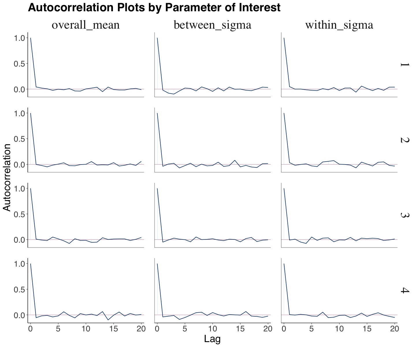
We can automatically display the correlation plot via mcmc_acf() from bayesplot. The $y$-axis indicates the autocorrelation function (ACF), for which 0 indicates no autocorrelation and 1 indicates full autocorrelation. The $x$-axis indicates the lag, i.e., how many steps apart the posterior samples are in the random walk.

lag_4_chains <- mcmc_acf(posterior_spotify_4_chains,
  pars = c(
    "overall_mean",
    "between_sigma",
    "within_sigma")
  ) +
  ggtitle("Autocorrelation Plots by Parameter of Interest") +
  theme(
    plot.title = element_text(size = 24, face = "bold", family = "sans"),
    axis.text = element_text(size = 17, family = "sans"),
    axis.title = element_text(size = 21, family = "sans"),
    legend.text = element_text(size = 17, family = "sans"),
    legend.title = element_text(size = 17, family = "sans")
  ) +
  facet_text(size = 26)

For the Spotify case, the autocorrelation significantly decreases before lag 5; this is a sign of a quick mixing (i.e., the chain is fast-moving around a well-defined parameter space of posterior values).

lag_4_chains

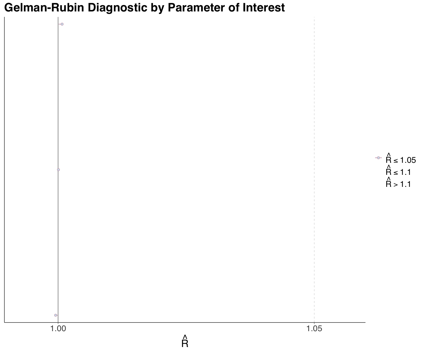
../_images/c723fe8af70ea9370a45b729d8309fd4033d95b29fcd2c4698482c0bf51b2c06.png

3.5. The Gelman-Rubin Diagnostic#

To evaluate within and between-chain sampling variability, we can use the Gelman-Rubin diagnostic known as $\hat{R}$. The intuition is that if our MCMC algorithm is working well, and if we run multiple copies of our chain, then they should all give us roughly the same answer.

In particular, we check that quantities related to the variance within each chain and variance between chains are roughly the same.

For a given parameter $\theta$ of interest, for which we run an MCMC simulation with $C$ chains, we let $\text{Var}_{\text{combined}}$ be the variabilty in the posterior samples of $\theta$ across our $C$ chains all combined and $\text{Var}_{\text{within}}$ the average variability in the posterior samples of $\theta$ in a standalone chain. The metric $\hat{R}$ is the following:

\[ \hat{R} \approx \sqrt{\frac{\text{Var}_{\text{combined}}}{\text{Var}_{\text{within}}}}. \]

Per parameter in our MCMC simulation, a given value of $\hat{R}$ indicates the following:

$\hat{R} \approx 1$ indicates stability across the $C$ chains.
$\hat{R} > 1$ indicates instability in the variability across all combined chains when compared to the average variability in a standalone chain.

We can automatically obtain this metric by parameter via rhat() from bayesplot.

spotify_r_hats <- rhat(posterior_spotify_4_chains,
  pars = c(
    "overall_mean",
    "between_sigma",
    "within_sigma"
  )
)
round(spotify_r_hats, 3)

overall_mean: 1
between_sigma: 1
within_sigma: 1.001

We do not have any major concerns regarding this metric for the Spotify case. We can also plot them via mcmc_rhat().

r_hats_4_chains <- mcmc_rhat(spotify_r_hats, size = 2) +
  ggtitle("Gelman-Rubin Diagnostic by Parameter of Interest") +
  theme(
    plot.title = element_text(size = 24, face = "bold", family = "sans"),
    axis.text = element_text(size = 17, family = "sans"),
    axis.title = element_text(size = 21, family = "sans"),
    legend.text = element_text(size = 17, family = "sans"),
    legend.title = element_text(size = 17, family = "sans")
  ) +
  facet_text(size = 26)

r_hats_4_chains

../_images/6d2a509c1463fca9064dfe6df08a3b604e48cc7a6f6c3c2eef8cb38b00704050.png

Exercise 25

Suppose you ran $C$ chains ($C > 1$) and have ensured all MCMC diagnostics are OK for all your parameters of interest.

What shall we do with all the resulting posterior samples, coming from all $C$ chains, when drawing our final inferential conclusions?

4. Wrapping Up#

Well, this is the end of a pretty interesting Bayesian journey (for now, in MDS).
Throughout these weeks, we have explored a new way of performing inference and prediction (sometimes via regression models) using foundational probability concepts and simulations. Priors, likelihood, and posteriors are always a must here.
The Bayesian paradigm is a vast field in Statistics and Machine Learning. You have the foundational tools to dig more into it from now on.