Lecture 1 - Frequentist and Bayesian Overview, Probabilistic Generative Models, and Stan

High-Level Goals of this Course

• Use Bayesian reasoning when modeling data.

• Apply Bayesian statistics to regression models.

• Compare and contrast Bayesian and frequentist methods, and evaluate their relative strengths.

• Use appropriate statistical libraries and packages for performing Bayesian inference.

Course Overview

• Non-project MDS course: eight lectures and four labs.

• Our focus is model-building, computation, and interpretation of results.

• We will build models in Stan along with rstan.

• Knowing how and when to use different statistical distributions is a great asset.

• R + Stan for lectures and labs.

Textbook

We will use a textbook in this course. Its name is Bayes Rules! An Introduction to Applied Bayesian Modeling). We will be posting suggested and optional readings of this book before our lecture time.

Today’s Learning Objectives

1. Review statistical inference (frequentist so far!).

2. Pave the way to Bayesian statistics.

3. Introduce probabilistic generative models.

4. Illustrate the basic use of Stan and rstan via Monte Carlo simulations.

5. Differentiate probability and likelihood in Statistics.

Loading Libraries

library(tidyverse)
library(infer)
library(tidyverse)
library(cowplot)
library(datateachr)
library(bayesrules)

1. Review of Frequentist Statistical Inference

In the frequentist courses, we have used observed data (coming from a random sample) to estimate and characterize uncertainty in unknown (or latent) population quantities of interest. For instance:

• An unknown population mean \(\mu\).

• An unknown population variance \(\sigma^2\).

• An unknown population median \(\text{M}\).

However, what do we mean when we say latent population quantities? Let us find it out.

1.1. Latent Variables

These latent quantities may be real but not directly observable. Hence, they are linked to other observable variables. For example:

• Using online ad click data to estimate the total lifetime revenue.

• Using genome sequencing to infer the origin of a virus during an outbreak.

• Using robotic Light Detection and Ranging (LiDAR) sensors to estimate the robot’s position.

Or completely hypothetical:

• Using tennis game win/loss data to infer a ranking of players.

• Using text data to learn the underlying hierarchy of topics.

Important

For these inquiries, the frequentist statistician’s usual hammers are point estimates and confidence intervals.

1.2. Why Care About Uncertainty?

Cannot we just collect more data?

Not if it is expensive (e.g., rocket telemetry), fundamentally limited (e.g., robot odometry), or outright impossible (e.g., ancestral species).

1.3. What is a Confidence Interval (CI)?

If we care about uncertainty in a frequentist inferential approach, what is a confidence interval?

Let us start with the first in-class question.

Exercise 1

Answer TRUE or FALSE:

Assuming a random sample of size \(n\) composed of the random variables \(X_1, X_2, \dots, X_n\) (not observed sampled values!), a frequentist 90%-confidence interval (CI) is a random interval that contains an unknown fixed population parameter of interest with probability 90% before observing the random data.

A. TRUE

B. FALSE

Exercise 2

A CI Example with Heights

Suppose I measure the height \(X_i\) (\(i=1, 2, \dots, n\)) of a simple randomly selected (i.e., all subjects have the same probability of being selected) subset of students in this room. My population of interest is the current MDS cohort.

Assume I know our true population standard deviation \(\sigma\), and I want to estimate our unknown mean \(\mu\) with the sample mean

\[\bar X = \frac{1}{n}\sum_{i=1}^n X_i.\]

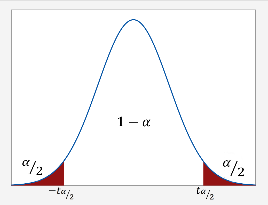
I design my 95% confidence interval using the Central Limit Theorem (CLT) formula:

\[\bar X - 1.96 \frac{\sigma}{\sqrt{n}} \leq \mu \leq \bar X + 1.96 \frac{\sigma }{\sqrt{n}},\]

where \(1.96\) is the \(0.975\)-quantile of the Standard Normal distribution.

Is this a valid confidence interval for \(\mu\)?

A. Yes.

B. No.

Now, let us proceed with an open-ended question.

Exercise 3

A Financial CI Example

Say you collect some yearly log returns \(X_1, \dots, X_n\) for a financial asset, and use \(\bar X = \frac{1}{n}\sum_{i=1}^n X_i\) to estimate the population mean.

But real log returns exhibit “very large/small values” much more frequently than a Normal distribution would predict. Your boss knows this and says:

“I know what we’ll do! We’ll model each \(X_i\) with a Cauchy distribution.”

Therefore, you might (well…) be able to compute a more suitable CI.

Nevertheless, you realize that Cauchy distributions have an undefined variance!

How do you compute a confidence interval?

Important

As a final thought now, before getting into our Bayesian introduction:

Even a minor change to a simple problem makes things significantly harder for frequentist methods!!!!!

2. Bayesian Statistics

The Bayesian statistical approach addresses these challenges.

• Very flexible, handles most analysis settings.

  • Missing data, non-standard data types, non-iid, weird loss functions, adding expert knowledge.

  • Every problem is the same, but your computer might disagree…

• Valid inference for any (finite) amount of data.

• Now the population parameters of interest are random variables! They have prior and posterior distributions.

• Easy to interpret uncertainty for the population parameters.

• Posterior distribution is a “one-stop-shop” for prediction, inference, decision-making, etc.

• Recursive updating.

What is recursive updating?

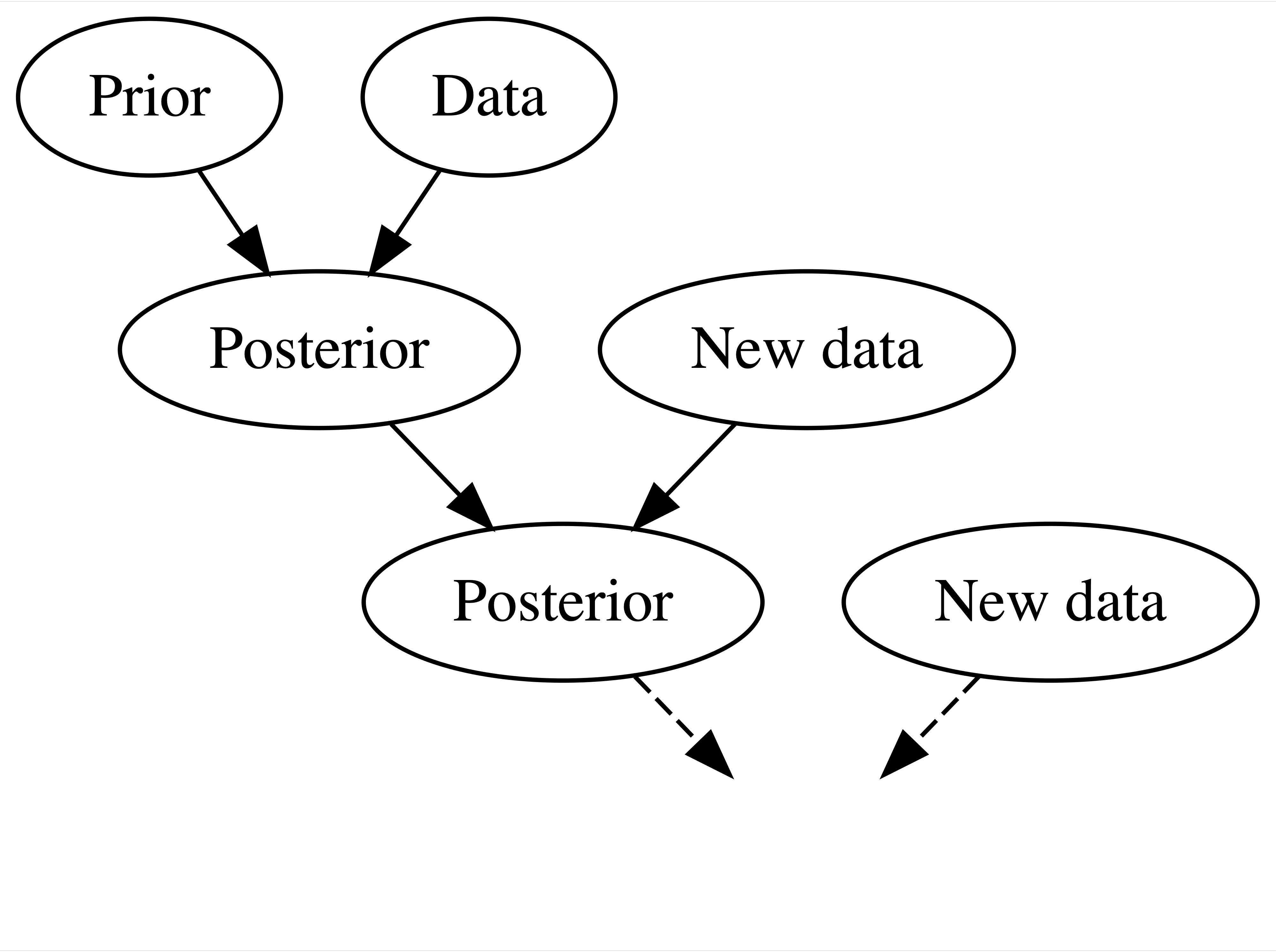
Source: Johnson et al. (2021)

Let us put this concept with an example of an Italian restaurant:

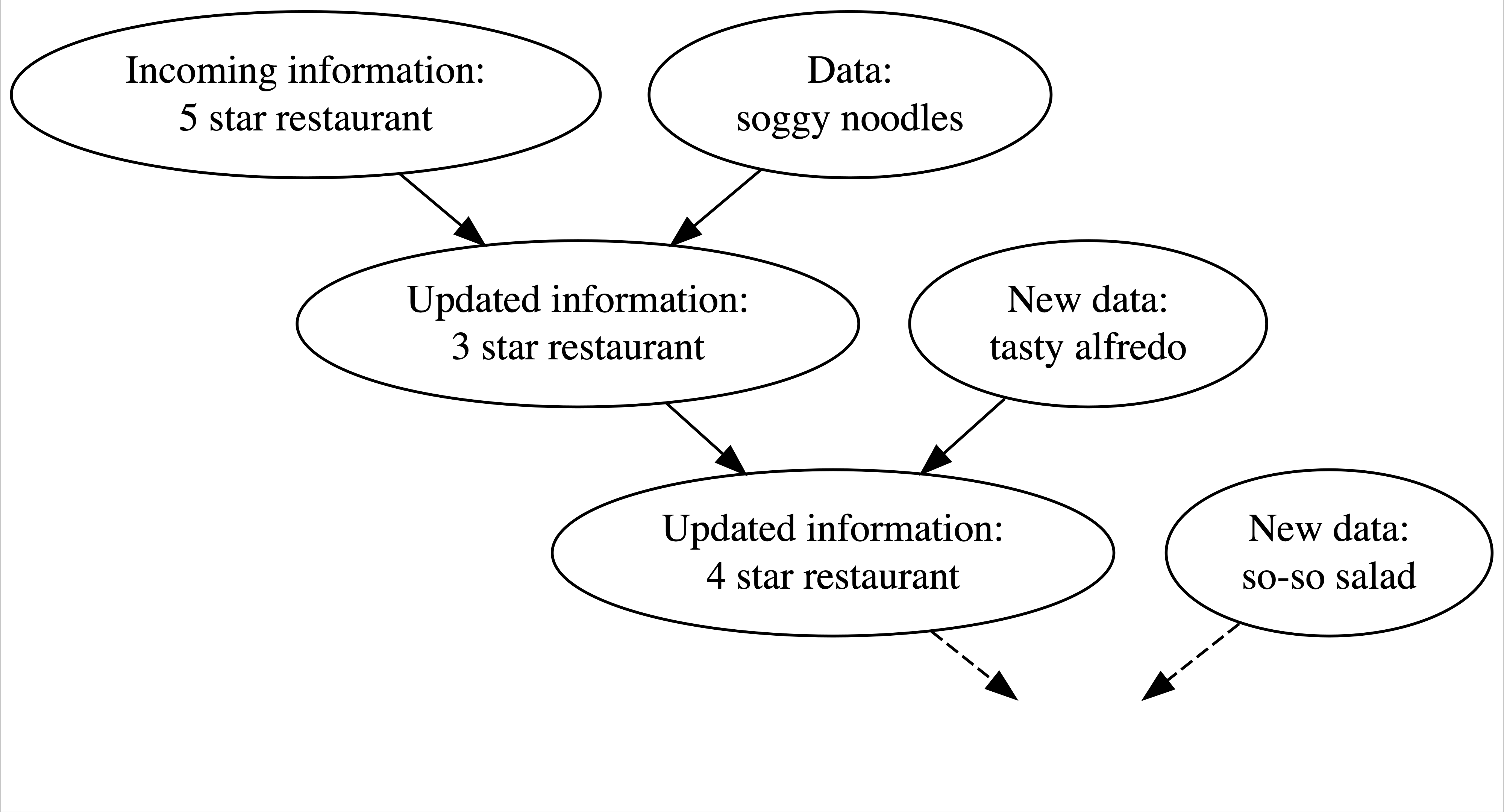
Source: Johnson et al. (2021)

Attention

Nonetheless, there is no free lunch…

• We would often need to be much more careful about computation.

• It requires slightly more model design work (prior).

• Less widely used in some areas of practice, e.g., medicine.

  • This is changing over time!

3. Generative Models

• For both frequentist and Bayesian statistics, a generative model is a simplified mathematical model for some reality: a “story about how your data were created.”

• The term generative means the model can be used to make synthetic data (i.e., running computational simulations!)

3.1. First Example

Newton’s laws of dynamics \(F = m \times a\) can be used to simulate position versus time given forces.

• What if I had noisy measurements of \(F\), \(m\), and \(a\) and wanted to infer their true values?

3.2. Second Example

We can model \(f(\cdot)\) for whether it will rain today given a vector of conditions/features \(\mathbf{X}\), \(f(\mathbf{X}) \to \{\text{yes}, \text{no}\}\). What class of response is \(f(\mathbf{X})\)?

\(f(\mathbf{X})\) is Bernoulli type!

Nonetheless, we cannot account for everything. Maybe only temperature, pressure, cloud cover, etc. Then, how do we deal with uncertainty in rain even under same measured conditions?

We can incorporate randomness into this model! This is analogous to \(\varepsilon\) on the right-hand side of a Ordinary Least-Squares (OLS) regression equation.

3.3. Probabilistic Generative Models

These models incorporate randomness into the system of interest. We design them using probability theory to add wiggle room to everything:

• We can incorporate noise in measurements (e.g., outputs coming from the \(F = m \times a\) model).

• They can be overly simplified models with incomplete measurements (e.g., rainy day model).

• They can even incorporate unobservable latent variables (e.g., hypothetical tennis rankings).

3.4. A Probabilistic Generative Model with a Bottle Cap Flip

You have arrived early to a movie with a friend, and have great seats. However, both of you need to use the washroom. Initially, you decide to flip a coin to see who gets to go first and who will watch the seats.

But it is 2025 and nobody carries coins any more! All you have is a bottle cap from your drink:

Let us start with a FREQUENTIST inferential problem:

What is the probability \(\pi\) the bottle cap will land right side up? We can use \(n\) trial tosses as data.

Attention

Let us reflect about the implications of using \(n\) trial tosses as data. We will obtain an estimate \(\hat{\pi}\) as a relative frequency coming from this data. Hence, the name frequentist.

The Math of Generative Model for a Bottle Cap Flip

Any probabilistic generative model involves setting up your random variable of interest along with your assumed distribution.

Thus, we have the following:

\[X_i \sim \mathrm{Bernoulli}(\pi) \quad \text{for} \quad i = 1, \dots, n.\]

• \(\pi \in [0, 1]\) is the unknown parameter we want to estimate: the probability the bottle cap will land right side up.

• \(X_i\) are the results of each bottle cap toss (\(1 = \text{right side up}\) or \(0 = \text{upside down}\)).

• \(X_i = 1\) is the success with probability \(\pi\).

The Bernoulli approach is a basic model for this case; we could design another more complex probabilistic model that considers initial conditions, wind, and collisions!

4. Stan and rstan Basics

The bottle cap example was set up as a FREQUENTIST inferential problem (an unknown FIXED parameter \(\pi\) we aim to estimate). This probabilistic generative model is a Bernoulli trial.

Since the frequentist approach relies on repeating this bottle cap toss many times to estimate \(\pi\), i.e., \(n \rightarrow \infty\) (not feasible to do it during our lecture time!), we will computationally simulate this system with a Monte Carlo simulation in a worksheet (not for marks) during lab1.

By definition, a Monte Carlo simulation will computationally repeat the event of interest \(n\) times with random inputs to obtain our \(n\) outputs of interest (a binary outcome in this case).

We can easily do this via the base R function rbernoulli() from purrr. But we will use this example to introduce Stan and rstan.

Stan is a probabilistic C++-based programming language for Bayesian statistical inference (but it can also perform simple Monte Carlo simulations). The R package rstan will allow pulling the simulation outputs from Stan.

4.1. Coding the Model and Running your Simulation

In general, we will follow these steps:

1. Code up our generative model in Stan.

2. Specify observed values of data to estimate using rstan (not necessary for Monte Carlo simulations).

3. Generate synthetic data.

4. Perform inference with your simulation outputs.

The generative model is all you need (and all you get!)

• Once you have a generative model, you can derive everything: tests, inference, etc.

• If your model can generate it, it will be handled in inference:

  • missing data, dependence, complex data types, etc.

• If your model cannot generate it, it will not be handled.

4.2. Can We Theoretically Estimate \(\pi\)?

Yes, we can! Maximum likelihood estimation (MLE) is the standard frequentist approach. Recall the procedure from DSCI 551’s lecture7.

How do we find the maximum likelihood estimate for \(\pi\) between 0 and 1?

• We set up the Bernoulli trial for one toss:

\[\mathscr{l}(\pi \mid x_i) = P(X_i = x_i \mid \pi) = \pi^{x_i}(1 - \pi)^{1 - x_i} \quad \text{for} \quad x_i = 0, 1.\]

• We obtain the joint likelihood function with \(n\) iid tosses:

\[\begin{split}\begin{align*} \mathscr{l}(\pi \mid x_1, \dots, x_n) &= \prod_{i=1}^n \pi^{x_i}(1 - \pi)^{1 - x_i} \\ &= \pi^{\sum_{i = 1}^n x_i}(1 - \pi)^{n - \sum_{i = 1}^n x_i}. \end{align*}\end{split}\]

• Then, the log-likelihood function:

\[ \log \mathscr{l}(\pi \mid x_1, \dots, x_n) = \sum_{i = 1}^n x_i \log(\pi) + \bigg(n - \sum_{i = 1}^n x_i \bigg) \log(1 - \pi). \]

• We take the first partial derivative of the log-likelihood function with respect to \(\pi\), set it to 0, and solve for \(\pi\):

\[\hat \pi = \frac{1}{n}\sum_{i=1}^n X_i.\]

4.3. Uncertainty in \(\pi\)

How can we characterize the uncertainty in \(\pi\) (without doing boatloads of math)?

A bootstrap CI might be the answer, but what if we only have \(n = 10\) replicates?

options(repr.matrix.max.rows = 10)
library(purrr)
library(tidyverse)
library(infer)

# Obtaining sample of size n = 10
set.seed(553)
sample_n10 <- tibble(flip = as.character(rbernoulli(n = 10, p = 0.7)))
sample_n10

Warning message:
“`rbernoulli()` was deprecated in purrr 1.0.0.”

A tibble: 10 × 1

flip
<chr>
TRUE
TRUE
TRUE
TRUE
TRUE
TRUE
TRUE
TRUE
FALSE
TRUE

# Obtaining bootstrap distribution via infer
set.seed(553)
bootstrap_distribution <- sample_n10 |>
  specify(response = flip, success = "TRUE") |>
  generate(reps = 1000, type = "bootstrap") |>
  calculate(stat = "prop")
mean_stat <- mean(bootstrap_distribution$stat)
mean_stat

# Obtainig percentile 95% CI
percentile_CI <- bootstrap_distribution |>
  get_confidence_interval(level = 0.95, type = "percentile")
percentile_CI

0.8967

A tibble: 1 × 2

lower_ci	upper_ci
<dbl>	<dbl>
0.7	1

options(repr.plot.height = 7, repr.plot.width = 12)

bootstrap_plot <- bootstrap_distribution |>
  visualize(bins = 6) + 
  shade_confidence_interval(endpoints = percentile_CI) +
  geom_vline(xintercept = mean_stat, linetype = "dashed") +
  theme(
    plot.title = element_text(size = 24, face = "bold"),
    axis.text = element_text(size = 17),
    axis.title = element_text(size = 21)
  ) +
  labs(x = "Statistic", y = "Count")

bootstrap_plot

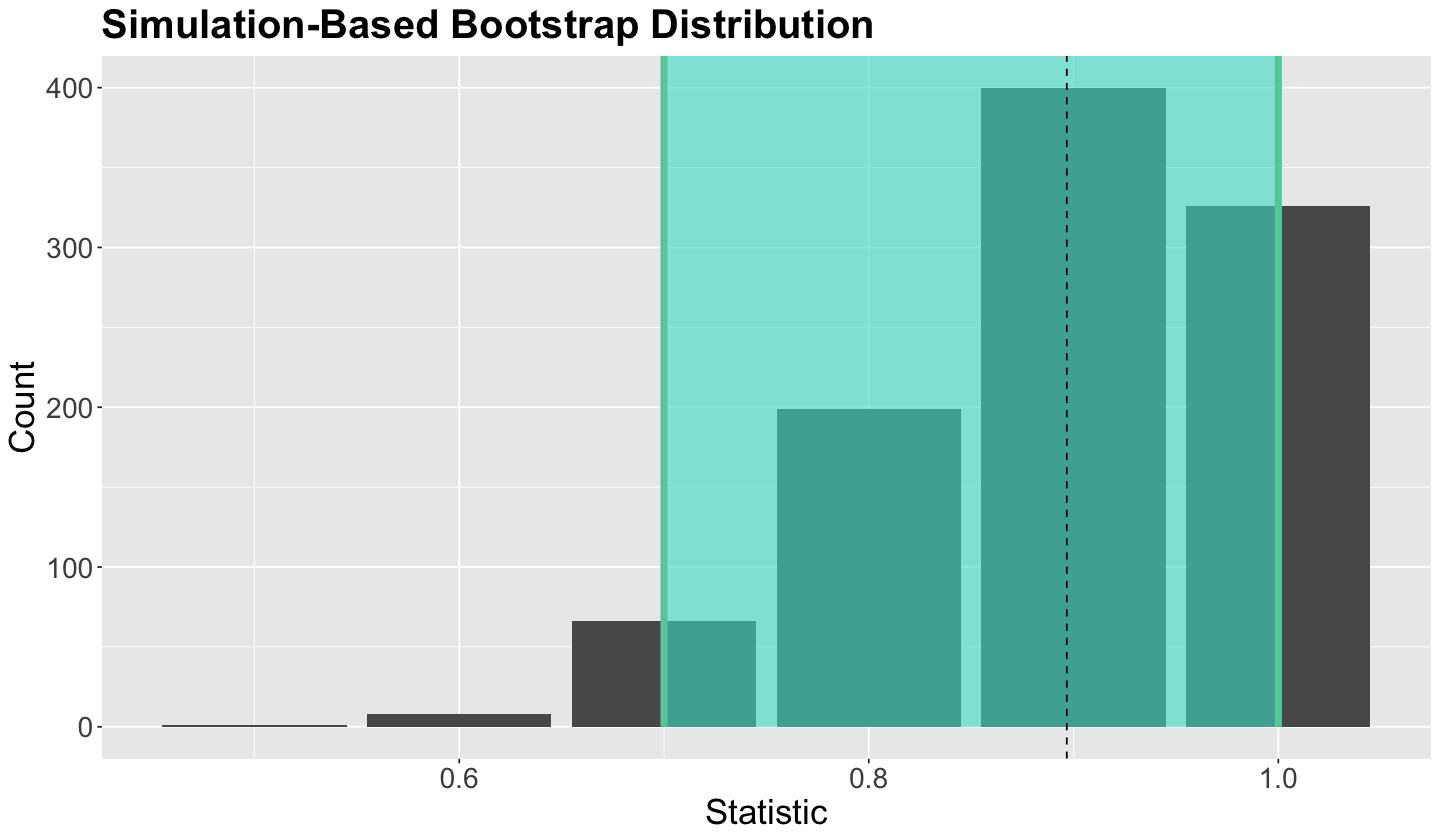
Important

Our 95% bootstrap CI shows biased results; the lower bound is 0.7! This is not good from an inferential perspective. An easy solution would be increasing the sample size \(n\), but what if this is not possible?

Bayesian inference will open up our set of possible solutions to this matter.

5. Difference between Probability and Likelihood

It is important to emphasize that in Statistics, probability and likelihood are NOT the same. In general, probability refers to the chance that some outcome of interest will happen for a particular random variable. Note a probability is always bounded between \(0\) and \(1\). Conversely, given some observed data, a likelihood refers to how plausible a given distributional parameter is. Furthermore, a likelihood is not bounded between \(0\) and \(1\).

Let us explore this concept via the Binomial distribution. Let \(X\) be the number of succcesses after \(n\) independent Bernoulli trials with probability of success \(0 \leq \pi \leq 1\). Then, \(X\) is said to have a Binomial distribution:

\[X \sim \text{Binomial} \left( n, \pi \right).\]

A Binomial distribution is characterized by the probability mass function (PMF)

(1)\[P \left(X = x \mid n, \pi \right) = {n \choose x} \pi^x (1 - \pi)^{n - x} \quad \text{for} \quad x = 0, 1, \dots, n.\]

Term \({n \choose x}\) indicates the total number of combinations for \(x\) successes out of \(n\) trials:

\[{n \choose x} = \frac{n!}{x!(n - x)!}.\]

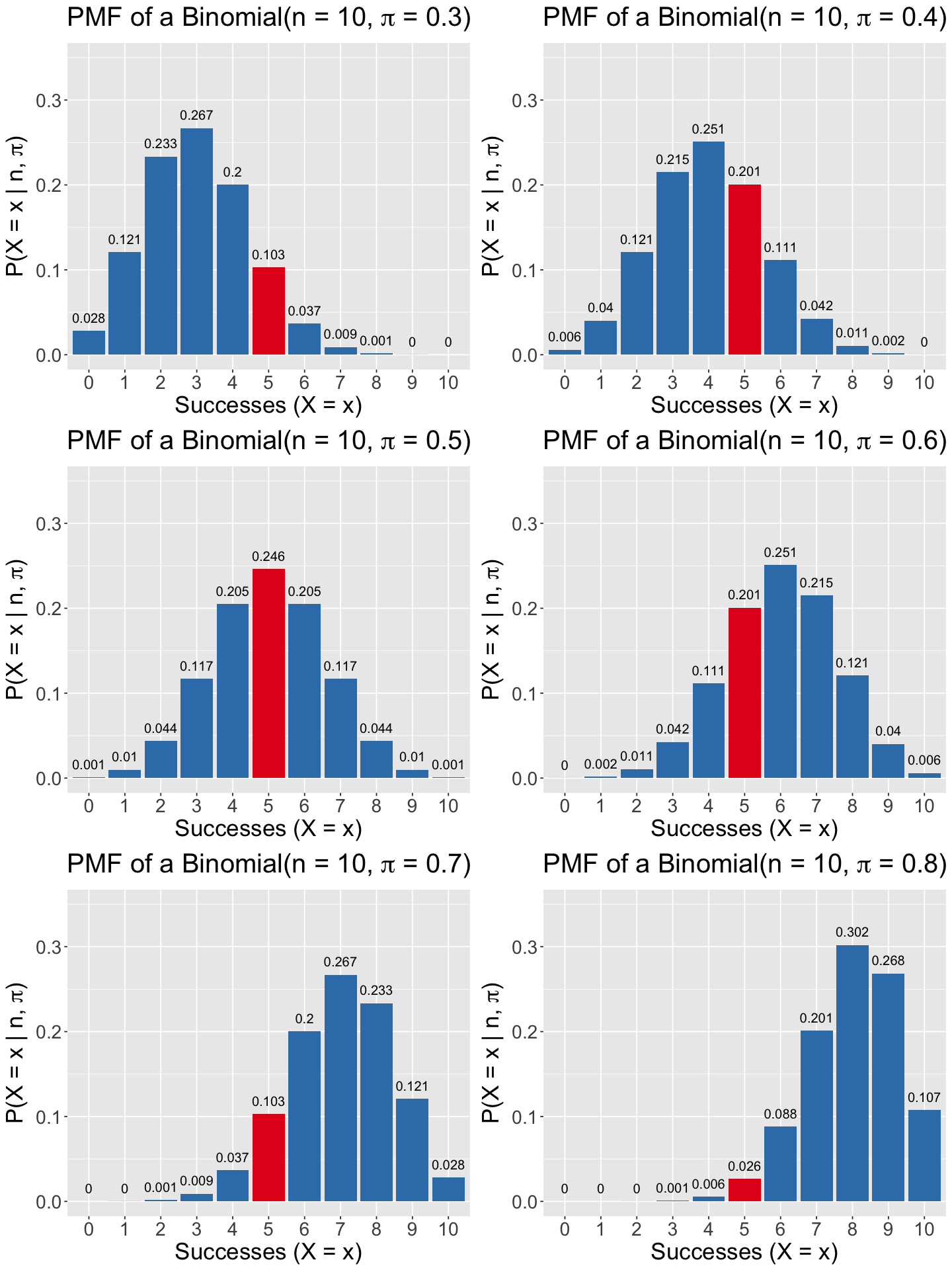
Let us plot the PMFs of six Binomial random variables. Note these plots indicate a probability \(P \left( X = x \mid n, \pi \right)\) on their \(y\)-axes and they have the same number of trials \(n = 10\):

• \(n = 10\) and \(\pi = 0.3\).

• \(n = 10\) and \(\pi = 0.4\).

• \(n = 10\) and \(\pi = 0.5\).

• \(n = 10\) and \(\pi = 0.6\).

• \(n = 10\) and \(\pi = 0.7\).

• \(n = 10\) and \(\pi = 0.8\).

Suppose we are specifically interested in the outcome \(Y = 5\), highlighted as a red bar in the six PMFs. We also indicate the probabilities associated to each outcome on top of each bar.

Suppose we sample data from a given Binomial population of interest, and this sample is composed of \(n = 10\) trials and \(x = 5\) successes. Under a frequentist paradigm, we are interested in inferring that value of \(\pi\), which is the most likely for these values of \(n\) and \(x\). Then, this is what we can do:

• Our PMF (1) will become a likelihood function given \(n = 10\) and our observed \(x = 5\) successes (note the lowercase \(x\)):

(2)\[\begin{split}\begin{align*} \mathscr{l}(\pi \mid x = 5, n = 10) &= P \left(X = 5 \mid n = 10, \pi \right) \\ &= {10 \choose 5} \pi^5 (1 - \pi)^{10 - 5}. \end{align*}\end{split}\]

Attention

The likelihood (2) is mathematically equal to the Binomial PMF with \(n = 10\) and \(X = 5\). Nevertheless, this likelihood is now in function of the parameter \(\pi\).

• That said, the below plot shows the likelihood function (2) with the plausible range of \(\pi\) on the \(x\)-axis (which is bounded between \(0\) and \(1\) since it is the probability of success in the Binomial distribution). Moreover, the likelihood values are indicated in the \(y\)-axis.

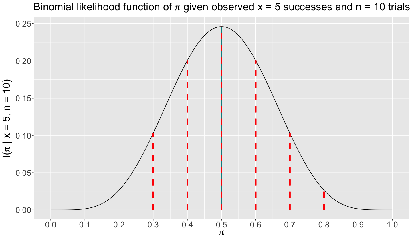
In the above likelihood plot, we highlighted as red vertical dashed lines those values corresponding to the red bars in the previous six Binomial PMFs (since a probability is MATHEMATICALLY equal to a likelihood, but not STATISTICALLY).

The plot shows that the likelihood function (2) gets maximized when \(\pi = 0.5\). That said, given our observed collected sample with \(x = 5\) successes with \(n = 10\), a value of \(\pi = 0.5\) is the most plausible (or likely!) in this Binomial population.

6. Wrapping Up with Frequentist Drawbacks

• We cannot incorporate our “expert” intuition, probabilistically speaking.

• How do we use side information, e.g., results of flips from other bottle caps?

• Asymptotic tools tend not to work well with small amounts of data.