Lecture 5 - Bayesian Normal Linear Regression and Hypothesis Testing

Today’s Learning Objectives

1. Describe the basics of Bayesian Normal linear regression.

2. Explore and contrast Bayesian Normal linear regression versus Ordinary Least-Squares (OLS).

3. Retake the concept of the posterior credible interval in a Beta-Binomial framework.

4. Introduce one-sided hypothesis testing in a Beta-Binomial framework.

5. Relate the posterior credible interval with the two-sided hypothesis in a Beta-Binomial framework.

Loading R Packages

options(repr.matrix.max.rows = 6)
library(bayesrules)
library(ggplot2)
library(tidyverse)
library(rstantools)
library(cowplot)
library(broom)
library(extraDistr)
library(rstan)
library(broom.mixed)
library(bayesplot)
library(wesanderson)

Previously…

We have explored the Bayes’ rule via probability theory with discrete and continuous variables. Note we expanded this approach to the Beta-Binomial and Gamma-Poisson models, a conjunction of continuous and discrete distributions for our prior and likelihood components, respectively. We already defined an interval estimate in a Bayesian framework: the posterior credible interval. Nonetheless, we have not discussed how to perform Bayesian hypothesis testing yet.

Additionally, the bike-share (Lecture 4 - Markov Chain Monte Carlo, Stan, and Complex Bayesian Models) and baseball (lab2) problems provided further insights into something we have not formally defined: Bayesian regression.

Therefore, it is time to check Bayesian hypothesis testing and Normal regression.

1. Bayesian Normal Linear Regression

Even though we already worked with two cases that paved the way (baseball and bikeshare data) to regression analysis, we have not formally introduced the concept of Bayesian regression. However, now that we have the Bayesian inference foundations, we can start with regression modelling in variable frameworks we explored in DSCI 561 and 562.

The general ideas remain:

• We need to assess the association (or causation if that is the case) between a response \(Y\) and our \(k\) regressors \(X_1, \dots, X_k\).

• Or, we need to predict a new \(Y'\) with our trained model.

1.1. The bikes Dataset

The bayesrules package contains another more reduced version of the dataset we used for our case in lecture4. According to the package’s documentation, the description is the following:

Data on ridership among registered members of the Capital Bikeshare service in Washington, D.C.

The dataset contains \(n = 500\) observations and thirteen variables.

bikes

A data.frame: 500 × 13

date	season	year	month	day_of_week	weekend	holiday	temp_actual	temp_feel	humidity	windspeed	weather_cat	rides
<date>	<fct>	<int>	<fct>	<fct>	<lgl>	<fct>	<dbl>	<dbl>	<dbl>	<dbl>	<fct>	<int>
2011-01-01	winter	2011	Jan	Sat	TRUE	no	57.39952	64.72625	80.5833	10.74988	categ2	654
2011-01-03	winter	2011	Jan	Mon	FALSE	no	46.49166	49.04645	43.7273	16.63670	categ1	1229
2011-01-04	winter	2011	Jan	Tue	FALSE	no	46.76000	51.09098	59.0435	10.73983	categ1	1454
⋮	⋮	⋮	⋮	⋮	⋮	⋮	⋮	⋮	⋮	⋮	⋮	⋮
2012-12-29	winter	2012	Dec	Sat	TRUE	no	50.69598	53.81600	75.2917	8.333661	categ2	1182
2012-12-30	winter	2012	Dec	Sun	TRUE	no	50.88048	52.85300	48.3333	23.500518	categ1	1432
2012-12-31	winter	2012	Dec	Mon	FALSE	no	47.92848	52.11383	57.7500	10.374682	categ2	2290

We will work with the following variables:

• weekend: Whether or not the date falls on a weekend (TRUE or FALSE). It is a binary variable and one of the regressors.

• temp_feel: What the temperature feels like (degrees Fahrenheit). It is a continuous variable and one of the regressors.

• rides: The number of bikeshare rides. It is an integer-type variable and our response.

bikeshare_data <- bikes |>
  select(weekend, temp_feel, rides)
bikeshare_data

A data.frame: 500 × 3

weekend	temp_feel	rides
<lgl>	<dbl>	<int>
TRUE	64.72625	654
FALSE	49.04645	1229
FALSE	51.09098	1454
⋮	⋮	⋮
TRUE	53.81600	1182
TRUE	52.85300	1432
FALSE	52.11383	2290

Main statistical inquiries

Suppose we are interested in the following statistical inquiries:

1. How are weekend and temp_feel associated with rides?

2. Is there a numerical result that can quantify this association?

3. Can we predict the number of rides during a weekend with 75 degrees Fahrenheit? What is the prediction interval?

Exercise 15

Let us retake DSCI 562 topics under a frequentist approach; what regression modelling can approach the above inquiries?

A. A generalized linear model (GLM) such as Multinomial regression.

B. A GLM such as Ordinal Logistic regression.

C. A GLM such as Poisson regression.

D. Ordinary Least-squares (OLS).

Source: Univariate Distribution Relationships

1.2. Exploratory Data Analysis

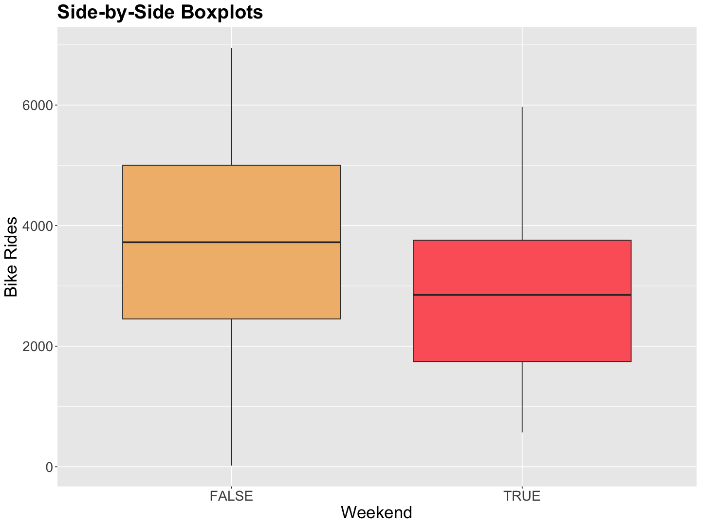
Let us make a quick exploratory data analysis on bikeshare_data: rides versus weekend and rides versus temp_feel.

options(repr.plot.height = 9, repr.plot.width = 12)

weekend_boxplots <- bikeshare_data |>
  ggplot(aes(weekend, rides)) +
  geom_boxplot(aes(fill = weekend)) +
  labs(y = "Bike Rides", x = "Weekend") +
  ggtitle("Side-by-Side Boxplots") +
  theme(
    plot.title = element_text(size = 24, face = "bold"),
    axis.text = element_text(size = 17),
    axis.title = element_text(size = 21),
    legend.position = "none"
  ) + 
  scale_fill_manual(values = wes_palette(n = 3, name = "GrandBudapest1"))

Note the bike rides tend to be less during weekends.

weekend_boxplots

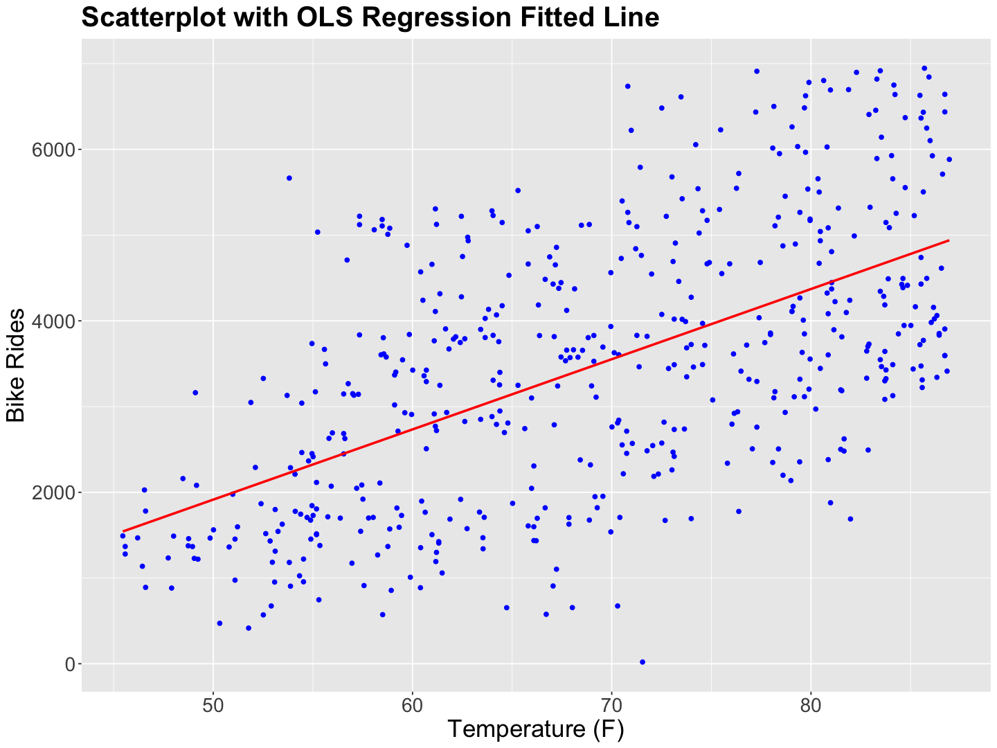
If we fit an OLS simple linear regression of temp_feel versus rides, the rides seem to increase along with temperature linearly.

bikeshare_data_scatterplot <- ggplot(bikeshare_data, aes(
  x = temp_feel, y = rides
)) +
  geom_point(color = "blue") +
  labs(y = "Bike Rides", x = "Temperature (F)") +
  geom_smooth(aes(temp_feel, rides), method = "lm", se = FALSE, colour = "red", formula = "y ~ x") +
  ggtitle("Scatterplot with OLS Regression Fitted Line") +
  theme(
    plot.title = element_text(size = 24, face = "bold"),
    axis.text.x = element_text(size = 17, angle = 0),
    axis.text.y = element_text(size = 17, angle = 0),
    axis.title = element_text(size = 21),
  )

bikeshare_data_scatterplot

1.3. Fitting a Frequentist OLS Regression Model

First, for the sake of approach comparison with \(i = 1 , \dots , n\); we will estimate an OLS regression model. In this case (for the \(i\)th observation) let \(Y_i\) be rides, \(X_{i,1}\) be temp_feel, and

\[\begin{split}\begin{equation*} X_{i, 2} = \begin{cases} 1 \; \; \; \; \mbox{if } \texttt{weekend} \mbox{ is } \texttt{TRUE},\\ 0 \; \; \; \; \mbox{otherwise;} \end{cases} \end{equation*}\end{split}\]

the OLS model is:

\[ Y_i = \beta_0 + \beta_1 X_{i, 1} + \beta_2 X_{i, 2} + \varepsilon_i. \]

With the following assumptions:

\[\begin{split}\begin{gather*} \mathbb{E}(\varepsilon_i) = 0 \\ \text{Var}(\varepsilon_i) = \sigma^2 \\ \varepsilon_i \sim \mathcal{N}(0, \sigma^2) \\ \varepsilon_i \perp \!\!\! \perp \varepsilon_k \; \; \; \; \text{for} \; i \neq k \; \; \; \; \text{(independence)}. \end{gather*}\end{split}\]

rides_OLS <- lm(rides ~ temp_feel + weekend, data = bikeshare_data)
tidy(rides_OLS, conf.int = TRUE) |> 
  mutate_if(is.numeric, round, 3)

A tibble: 3 × 7

term	estimate	std.error	statistic	p.value	conf.low	conf.high
<chr>	<dbl>	<dbl>	<dbl>	<dbl>	<dbl>	<dbl>
(Intercept)	-1873.751	351.790	-5.326	0	-2564.929	-1182.573
temp_feel	80.347	4.971	16.162	0	70.580	90.115
weekendTRUE	-707.621	123.644	-5.723	0	-950.550	-464.693

Attention

From the frequentist point of view, the output indicates statistically significant coefficients. Note the estimated intercept is negative, which does not make sense for rides. We could fix this in our Bayesian approach.

1.4. Setting up a Bayesian Regression Model

Now that rides_OLS is all done, let us start our Bayesian model. Assuming response normality, we have the following:

\[Y_i \sim \mathcal{N}(\mu_i = \beta_0 + \beta_1 X_{i, 1} + \beta_2 X_{i, 2}, \sigma^2)\]

Important

Each \(Y_i\) will have its own mean \(\mu_i\). This mean is the systematic component of the regression model. Furthermore, all responses will share a common variance \(\sigma^2\) (analogous to the error terms in OLS).

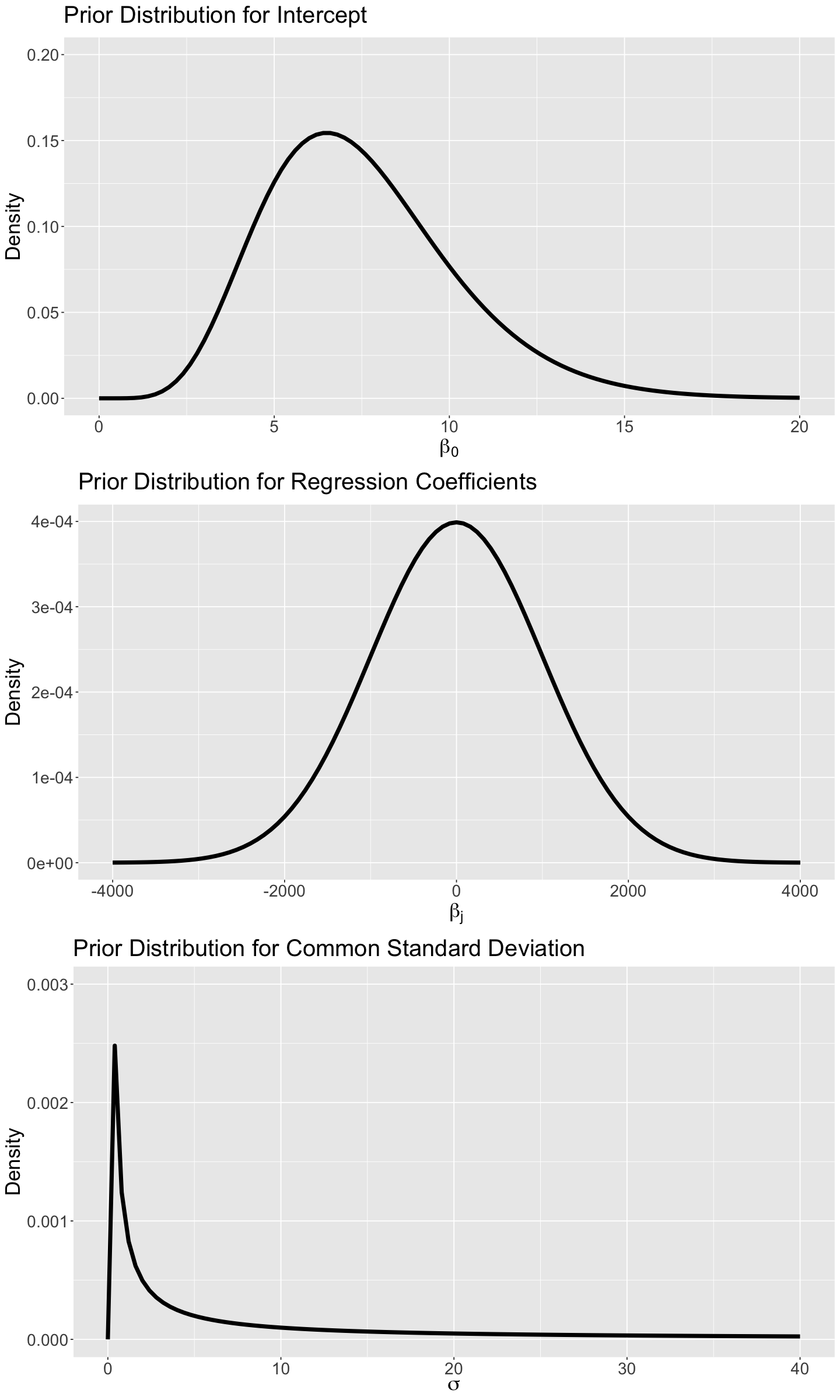
For the prior specification, we will proceed as follows:

• \(\beta_0 \sim \text{Gamma}(\alpha = 7.5, \beta = 1)\).

• \(\beta_1 \sim \mathcal{N}(\mu_{\beta_1} = 0, \sigma_{\beta_1}^2 = 1000^2)\).

• \(\beta_2 \sim \mathcal{N}(\mu_{\beta_2} = 0, \sigma_{\beta_2}^2 = 1000^2)\).

• \(\sigma \sim \mathrm{IG}(\eta = 0.001, \lambda = 0.001)\), this is the Inverse Gamma distribution parametrized by shape \(\eta = 0.001\) and rate \(\lambda = 0.001\). This prior distribution is a popular choice for \(\sigma > 0\). The Stan syntax is available here.

Attention

We have to stress the following:

• For these prior specifications, we assume that the mean of the \(\beta_j\) (\(j = 1, 2\)) is \(0\), since we do not know if the variable \(X_{i,j}\) has any association with \(Y_i\). We will use a large variance (i.e, \(\sigma_{\beta_j}^2 = 1000^2\)) on the coefficients to reflect PRIOR uncertainty.

• We also specify a nonnegative prior distribution (i.e., Inverse Gamma) for the common variance of the error terms \(\sigma^2 > 0\).

• The nature of rides is non-negative. Hence, a Gamma prior on \(\beta_0\) makes more sense than a Normal. Its hyperparameters are chosen to reflect our uncertainty in this intercept.

The density plots for these priors are shown below.

# Plotting Gamma prior for a_w
prior_gamma_beta_0 <- ggplot() +
  xlim(0, 20) +
  ylim(0, 0.2) +
  geom_function(fun = dgamma, args = list(shape = 7.5, rate = 1), linewidth = 2) +
  theme(
    plot.title = element_text(size = 24, face = "bold"),
    axis.text.x = element_text(size = 17, angle = 0),
    axis.text.y = element_text(size = 17, angle = 0),
    axis.title = element_text(size = 21),
  ) +
  labs(y = "Density", x = expression(beta["0"])) +
  ggtitle(expression("Prior Distribution for Intercept"))

# Plotting Normal prior for regression coefficients
prior_gamma_beta_j <- ggplot() +
  xlim(-4000, 4000) +
  ylim(0, 0.0004) +
  geom_function(fun = dnorm, args = list(mean = 0, sd = 1000), linewidth = 2) +
  theme(
    plot.title = element_text(size = 24, face = "bold"),
    axis.text.x = element_text(size = 17, angle = 0),
    axis.text.y = element_text(size = 17, angle = 0),
    axis.title = element_text(size = 21),
  ) +
  labs(y = "Density", x = expression(beta["j"])) +
  ggtitle(expression("Prior Distribution for Regression Coefficients"))

# Plotting Inverted Gamma prior for common variance
prior_inverted_gamma_sigma_sq <- ggplot() +
  xlim(0, 40) +
  ylim(0, 0.003) +
  geom_function(fun = dinvgamma, args = list(alpha = 0.001, beta = 0.001), linewidth = 2) +
  theme(
    plot.title = element_text(size = 24, face = "bold"),
    axis.text.x = element_text(size = 17, angle = 0),
    axis.text.y = element_text(size = 17, angle = 0),
    axis.title = element_text(size = 21),
  ) +
  labs(y = "Density", x = expression(sigma)) +
  ggtitle(expression("Prior Distribution for Common Standard Deviation"))

options(repr.plot.height = 20, repr.plot.width = 12)

plot_grid(prior_gamma_beta_0, prior_gamma_beta_j, prior_inverted_gamma_sigma_sq, nrow = 3)

Finally, we formalize the model with a dataset containing \(n\) observations (i.e., rows in bikes), for the \(i\)th observation \((i = 1, \dots, n)\) with \(Y_i\) rides, \(X_{i,1}\) temp_feel and the dummy \(X_{i,2}\) for weekend:

\[\begin{split}\begin{align*} \text{likelihood:} \qquad Y_i \mid \beta_0, \beta_1, \beta_2, \sigma^2 \mathop\sim^\text{ind} \mathcal{N} (\mu_i, \sigma^2) \\ \text{where} \quad \mu_i = \beta_0 + \beta_1 X_{i, 1} + \beta_2 X_{i,2} \\ \text{priors:} \quad \beta_0 \sim \text{Gamma}(\alpha = 7.5, \beta = 1) \\ \beta_1 \sim \mathcal{N}(\mu_{\beta_1} = 0, \sigma_{\beta_1}^2 = 1000^2) \\ \beta_2 \sim \mathcal{N}(\mu_{\beta_2} = 0, \sigma_{\beta_1}^2 = 1000^2) \\ \sigma \sim \mathrm{IG}(\eta = 0.001, \lambda = 0.001). \end{align*}\end{split}\]

1.5. Markov Chain Monte Carlo Simulation

We proceed with the Stan code for this model. We will continue using the blocks data, parameters, and model.

Additionally, we introduce the block generated_quantities. This block is executed after obtaining our posterior samples for the parameters. The new block needs the variables pred_x_1 and pred_x_2 for the predictive inquiry for the weekend (pred_x_2) with 75 degrees Fahrenheit (pred_x_1). We input these variables in data.

Important

The block generated_quantities will create a posterior predictive distribution y_pred which takes into account two sources of variability:

• Posterior variability in parameters: We will generate one prediction by row from the Markov Chain Monte Carlo (MCMC) output to take into account this variability, i.e., the variability will come from our approximate joint posterior distribution. These predictions will be computed using the fixed values pred_x_1 and pred_x_2.

• Sampling variability: Each prediction by row from the MCMC output should deviate from its respective posterior prediction (computed with the posterior sampled parameters). Thus, we will add random noise to it.

We are basically constructing a predictive distribution for the response for a weekend with 75 degrees Fahrenheit, from which we will compute an interval analogous to the Prediction Interval (PI) from OLS.

The block generated quantities takes the posterior samples of our parameters and computes \(\mu_i\) with the fixed values pred_x_1 and pred_x_2. Then, we used a Normal random number generator normal_rng() to add the so-called random noise.

bikerides_stan <- "data {
  int<lower=0> n;                               // training sample size
  vector[n] y;                                  // response vector
  vector[n] x_1;                                // regressor 1 vector
  vector[n] x_2;                                // regressor 2 vector
  real pred_x_1;                                // fixed value for regressor 1
  real pred_x_2;                                // fixed value for regressor 2
}
parameters {
  real<lower=0> beta_0;                         // intercept with lower bound
  real beta_1;                                  // regression coefficient 1
  real beta_2;                                  // regression coefficient 2
  real<lower=0> sigma;                          // common standard deviation with lower bound
  }
model {
  beta_0 ~ gamma(7.5, 1);                       // alpha = 7.5 and beta = 1
  beta_1 ~ normal(0, 1000);                     // mu_b1 = 0 and sigma_b1 = 1000
  beta_2 ~ normal(0, 1000);                     // mu_b2 = 0 and sigma_b2 = 1000
  sigma ~ inv_gamma(0.001, 0.001);              // eta = 0.001 and lambda = 0.001
  y ~ normal(beta_0 + beta_1 * x_1 + beta_2 * x_2, sigma);
}
generated quantities {
  real y_pred = normal_rng(beta_0 + beta_1 * pred_x_1 + beta_2 * pred_x_2, sigma);
}"

Next, we create a dictionary with all the data variables we need to pass into Stan as a list(). We cannot pass logical values to Stan but 0s and 1s. Hence we use model_matrix() to convert column weekend to 0s and 1s.

model_matrix <- as.data.frame(model.matrix(rides ~ temp_feel + weekend, data = bikeshare_data))
model_matrix

bikerides_dictionary <- list(
  n = nrow(bikeshare_data), 
  y = bikeshare_data$rides,
  x_1 = bikeshare_data$temp_feel,
  x_2 = model_matrix$weekendTRUE,
  pred_x_1 = 75,
  pred_x_2 = 1
)

A data.frame: 500 × 3

	(Intercept)	temp_feel	weekendTRUE
	<dbl>	<dbl>	<dbl>
1	1	64.72625	1
2	1	49.04645	0
3	1	51.09098	0
⋮	⋮	⋮	⋮
498	1	53.81600	1
499	1	52.85300	1
500	1	52.11383	0

Then, we compile the Stan model and run the simulation.

posterior_bikeshare <- stan(
  model_code = bikerides_stan,
  data = bikerides_dictionary,
  chains = 1,
  iter = 40000,
  warmup = 20000,
  thin = 60,
  seed = 553,
)

SAMPLING FOR MODEL 'anon_model' NOW (CHAIN 1).
Chain 1: 
Chain 1: Gradient evaluation took 4.7e-05 seconds
Chain 1: 1000 transitions using 10 leapfrog steps per transition would take 0.47 seconds.
Chain 1: Adjust your expectations accordingly!
Chain 1: 
Chain 1: 
Chain 1: Iteration:     1 / 40000 [  0%]  (Warmup)
Chain 1: Iteration:  4000 / 40000 [ 10%]  (Warmup)
Chain 1: Iteration:  8000 / 40000 [ 20%]  (Warmup)
Chain 1: Iteration: 12000 / 40000 [ 30%]  (Warmup)
Chain 1: Iteration: 16000 / 40000 [ 40%]  (Warmup)
Chain 1: Iteration: 20000 / 40000 [ 50%]  (Warmup)
Chain 1: Iteration: 20001 / 40000 [ 50%]  (Sampling)
Chain 1: Iteration: 24000 / 40000 [ 60%]  (Sampling)
Chain 1: Iteration: 28000 / 40000 [ 70%]  (Sampling)
Chain 1: Iteration: 32000 / 40000 [ 80%]  (Sampling)
Chain 1: Iteration: 36000 / 40000 [ 90%]  (Sampling)
Chain 1: Iteration: 40000 / 40000 [100%]  (Sampling)
Chain 1: 
Chain 1:  Elapsed Time: 1.595 seconds (Warm-up)
Chain 1:                1.954 seconds (Sampling)
Chain 1:                3.549 seconds (Total)
Chain 1: 

1.6. Obtaining, Visualizing, and Interpreting the Posterior Results

When comparing both outputs, Bayesian and OLS, we highlight the following:

• Our nonnegative Bayesian intercept is more precise than the negative OLS estimation.

• Moreover, the point estimates for \(\beta_1\) differ greatly, but the Bayesian one is more precise (check the posterior credible interval versus the frequentist 95% confidence interval).

• Regarding the point estimates for \(\beta_2\), both approaches show considerable variability.

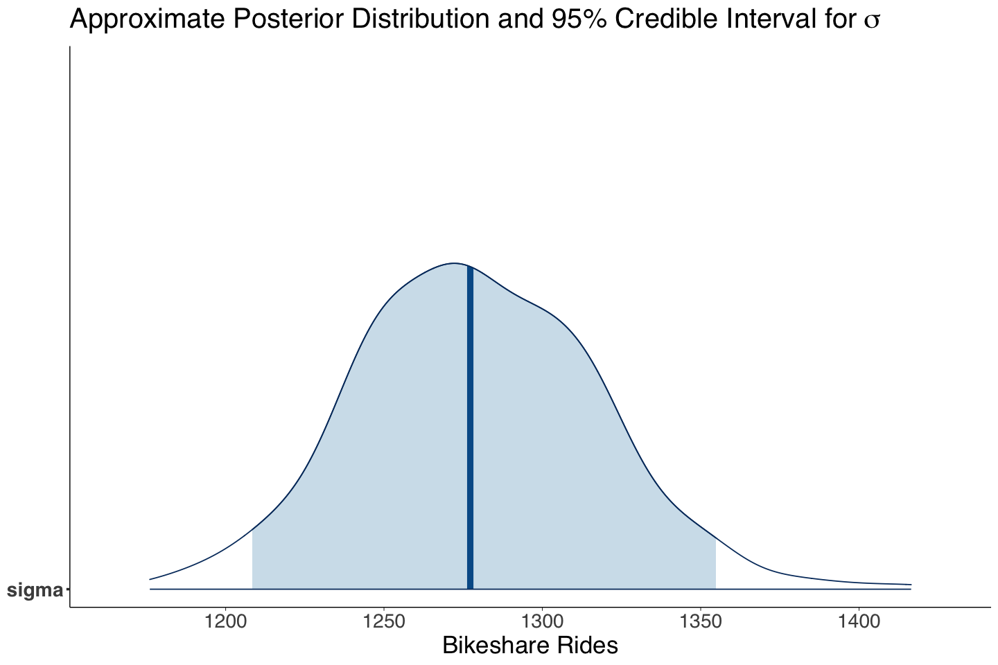
• Note that the point estimates for \(\sigma\) are quite similar between both approaches!

• Finally, both predictive intervals show high variability.

# Bayesian posterior summaries!
tidy_posterior_bikeshare <- round(summary(posterior_bikeshare)$summary, 2)[-6, c("mean", "sd", "2.5%", "97.5%")]
tidy_posterior_bikeshare

A matrix: 5 × 4 of type dbl

	mean	sd	2.5%	97.5%
beta_0	7.50	2.76	3.15	14.11
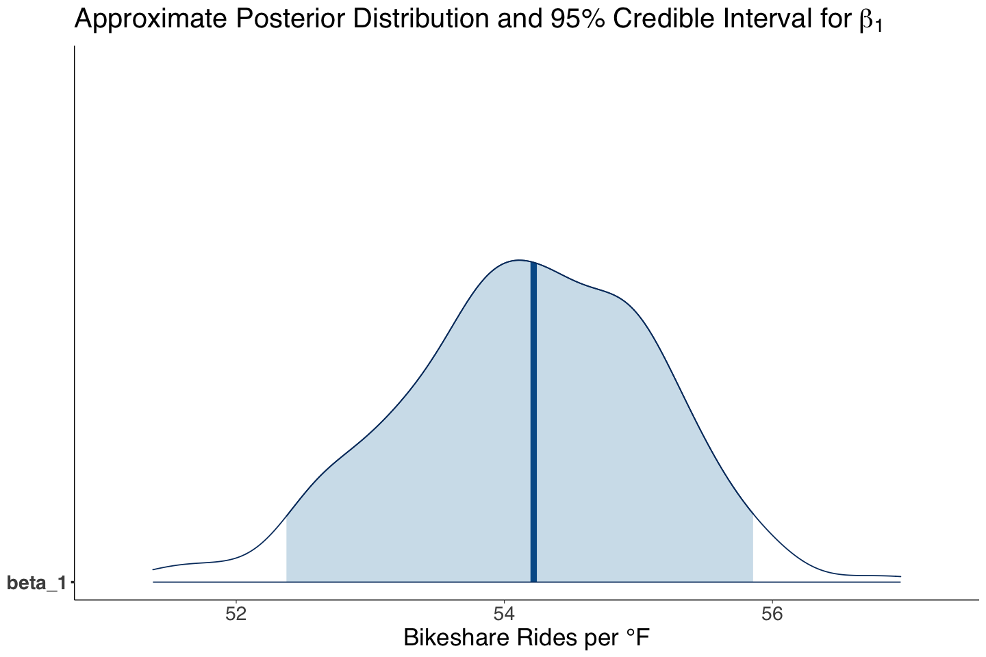
beta_1	54.17	0.94	52.37	55.86
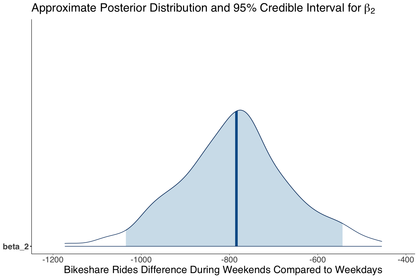
beta_2	-789.32	124.54	-1034.84	-543.73
sigma	1279.47	38.09	1208.41	1354.80
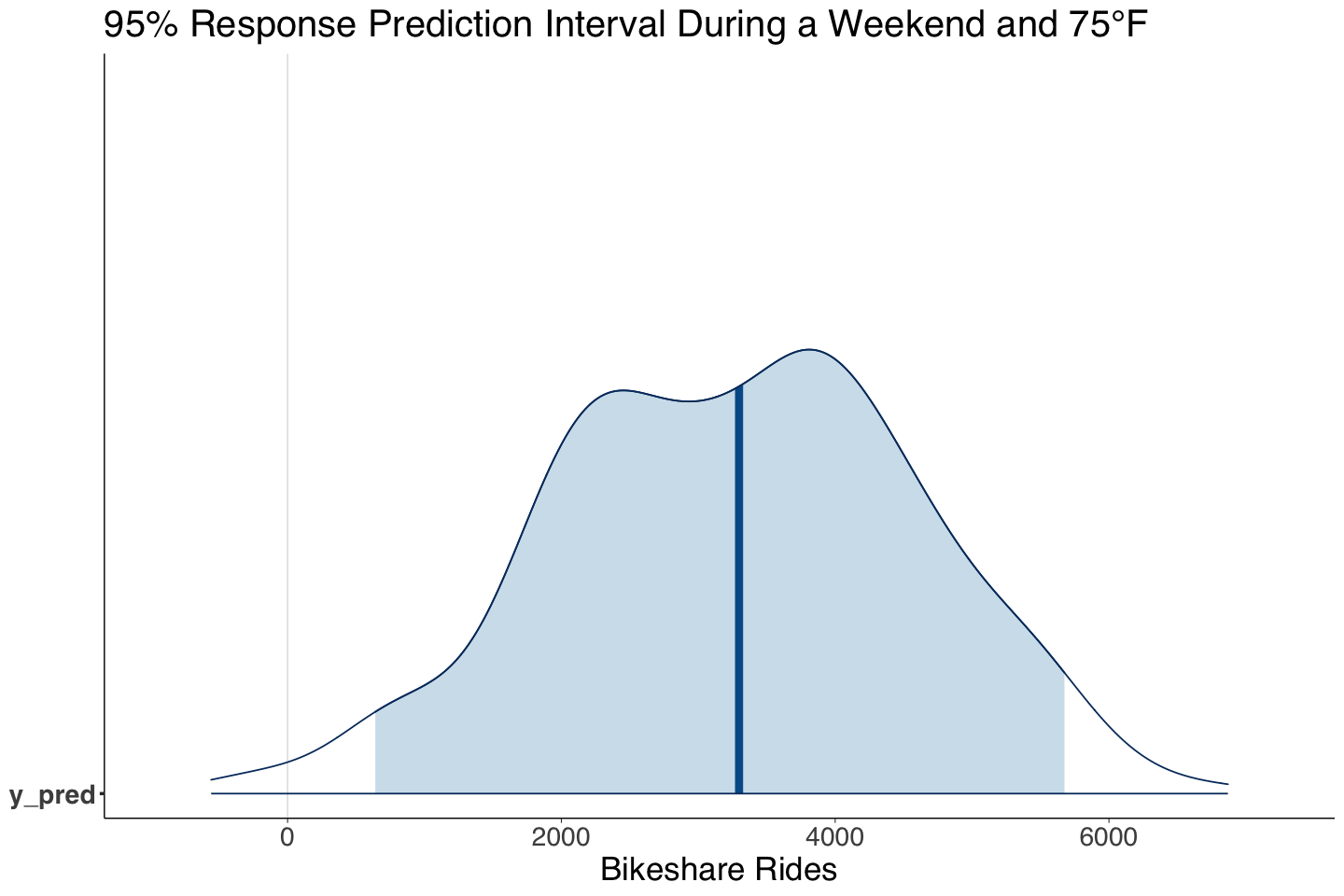
y_pred	3279.83	1332.33	640.81	5674.73

# Frequentist OLS output!
tidy(rides_OLS, conf.int = TRUE) |> 
  mutate_if(is.numeric, round, 3)
glance(rides_OLS) |> 
  mutate_if(is.numeric, round, 3)
predict.lm(rides_OLS, newdata = data.frame(temp_feel = 75, weekend = TRUE), interval = "prediction")

A tibble: 3 × 7

term	estimate	std.error	statistic	p.value	conf.low	conf.high
<chr>	<dbl>	<dbl>	<dbl>	<dbl>	<dbl>	<dbl>
(Intercept)	-1873.751	351.790	-5.326	0	-2564.929	-1182.573
temp_feel	80.347	4.971	16.162	0	70.580	90.115
weekendTRUE	-707.621	123.644	-5.723	0	-950.550	-464.693

A tibble: 1 × 12

r.squared	adj.r.squared	sigma	statistic	p.value	df	logLik	AIC	BIC	deviance	df.residual	nobs
<dbl>	<dbl>	<dbl>	<dbl>	<dbl>	<dbl>	<dbl>	<dbl>	<dbl>	<dbl>	<dbl>	<dbl>
0.38	0.378	1242.26	152.4	0	2	-4270.308	8548.617	8565.475	766974881	497	500

A matrix: 1 × 3 of type dbl

	fit	lwr	upr
1	3444.68	994.407	5894.953

Retaking our initial inquiries, we state the following:

1. How are weekend and temp_feel associated with rides?

2. Is there a numerical result that can quantify this association?

Our Bayesian estimates (i.e., means of the MCMC posterior samples) for \(\beta_1\) and \(\beta_2\) indicate that bike rides linearly increase by 54.20 on average for each degree Fahrenheit, whereas they decrease by 796.40 on average during weekends.

Statistically, according to our 95% posterior credible intervals, the regression coefficients are different from zero (the intervals do not contain it).

3. Can we predict the number of rides during a weekend with 75 degrees Fahrenheit? What is the prediction interval?

Yes, we can obtain a Bayesian posterior predictive distribution for a 95% prediction interval of the number of rides during a weekend with 75 degrees Fahrenheit:

\[(640.81, 5674.73).\]

Let us plot the aproximate posterior distribution for temp_feel (\(\beta_1\)):

options(repr.plot.height = 8, repr.plot.width = 12)

beta_1_post_dist <- mcmc_areas(posterior_bikeshare, pars = c("beta_1"), prob = 0.95) +
  theme(
    plot.title = element_text(size = 24, family = "sans"),
    axis.text.x = element_text(size = 17, angle = 0, family = "sans"),
    axis.text.y = element_text(size = 17, angle = 0, family = "sans"),
    axis.title = element_text(size = 21, family = "sans")
  ) +
  labs(title = expression("Approximate Posterior Distribution and 95% Credible Interval for" ~ beta[1])) +
  xlab("Bikeshare Rides per °F")

beta_1_post_dist

Now, we will do it for weekend (\(\beta_2\)):

beta_2_post_dist <- mcmc_areas(posterior_bikeshare, pars = c("beta_2"), prob = 0.95) +
  theme(
    plot.title = element_text(size = 24, family = "sans"),
    axis.text.x = element_text(size = 17, angle = 0, family = "sans"),
    axis.text.y = element_text(size = 17, angle = 0, family = "sans"),
    axis.title = element_text(size = 21, family = "sans")
  ) +
  labs(title = expression("Approximate Posterior Distribution and 95% Credible Interval for" ~ beta[2])) +
  xlab("Bikeshare Rides Difference During Weekends Compared to Weekdays")

beta_2_post_dist

Then, we proceed with \(\sigma\) (the overall standard deviation between the observations).

sigma_post_dist <- mcmc_areas(posterior_bikeshare, pars = c("sigma"), prob = 0.95) +
  theme(
    plot.title = element_text(size = 24, family = "sans"),
    axis.text.x = element_text(size = 17, angle = 0, family = "sans"),
    axis.text.y = element_text(size = 17, angle = 0, family = "sans"),
    axis.title = element_text(size = 21, family = "sans")
  ) +
  labs(title = expression("Approximate Posterior Distribution and 95% Credible Interval for" ~ sigma)) +
  xlab("Bikeshare Rides")

sigma_post_dist

And finally, the 95% prediction interval of the number of rides during a weekend with 75°F.

PI_post_dist <- mcmc_areas(posterior_bikeshare, pars = c("y_pred"), prob = 0.95) +
  theme(
    plot.title = element_text(size = 24, family = "sans"),
    axis.text.x = element_text(size = 17, angle = 0, family = "sans"),
    axis.text.y = element_text(size = 17, angle = 0, family = "sans"),
    axis.title = element_text(size = 21, family = "sans")
  ) +
  labs(title = "95% Response Prediction Interval During a Weekend and 75°F") +
  xlab("Bikeshare Rides")

PI_post_dist

Caution

The 95% credible and the prediction intervals, show a critical concern: large variability in MCMC sampling for \(\beta_2\), \(\sigma\), and the prediction interval. These findings suggest the model is not capturing the right systematic component, i.e., the relation might be non-linear, and there might be other regressors we are missing.

2. The Tinder Example Comes Back

We have had enough bottle cap flips on this block. So let us retake a new Tinder example while applying what we learned in the theoretical Beta-Binomial model from Lecture 3 - Bayesian Statistics in Action: The Beta-Binomial Model.

Again, for the single population living in Vancouver looking for a partner, let us suppose we want to make inference on the probability \(\pi\) of finding a partner when using Tinder.

Attention

This Tinder example is a whole new problem with different data. In Lecture 2 - Conditional Probabilities, Bayes’ Rule, and Maximum a Posteriori Estimation, we were building the intuition of the Bayes’ rule using Bernoulli distributions, without getting into Beta-Binomial terrains. But now, we can elaborate more formal Bayesian conclusions by using the Beta-Binomial model we saw in Lecture 3 - Bayesian Statistics in Action: The Beta-Binomial Model.

Let us recall the Bayes’ rule:

\[\text{posterior} \propto \text{prior} \times \text{likelihood}.\]

Hence, via new Tinder data, let us build our theoretical posterior before proceeding with Bayesian hypothesis testing.

2.1. The Prior

We need to obtain our Beta prior for \(\pi\). Again, as an enthusiastic Tinder researcher in the literature, I collected information from 60 previous studies on using this app to find a partner. These studies were run in cities as similar as Vancouver.

Furthermore, in each study, there was a sample of single subjects. All subjects were using Tinder in each sample. The corresponding researchers recorded how many subjects ended up partnered in each study by using Tinder (the success).

Warning

Again, this is simulated data.

Let us recall the Bernoulli trial we used in Lecture 3 - Bayesian Statistics in Action: The Beta-Binomial Model.

A independent subject \(X_i\) is assumed as:

\[X_i \sim \mathrm{Bernoulli}(\pi) \quad \text{for} \quad i = 1, \dots, n.\]

• \(\pi \in [0, 1]\) is the unknown parameter we want to infer: the probability of finding a partner if we use Tinder.

• \(X_i\) is the result at the end of the study (\(1 = \text{partnered}\) or \(0 = \text{non-partnered}\)).

• \(X_i = 1\) is the success with probability \(\pi\).

• \(n\) is the sample size of each study.

Now, we need to set our theoretical Beta prior. I recorded the estimation results of \(\pi\) in these 60 studies. It is stored in tinder_prior_pi_studies.

tinder_prior_pi_studies <- read_csv("../data/tinder_prior_pi_studies.csv", show_col_types = FALSE)
tinder_prior_pi_studies

A spec_tbl_df: 60 × 1

tinder_prior_pi
<dbl>
0.2652300
0.3879204
0.2221071
⋮
0.3726435
0.2260178
0.2890508

Now, we obtain a histogram of tinder_prior_pi_studies (with the \(y\)-axis adjusted as a after_stat(density)).

hist_prior <- ggplot() +
  geom_histogram(
    data = tinder_prior_pi_studies,
    aes(x = tinder_prior_pi, y = after_stat(density)), fill = "grey", color = "blue", bins = 7, alpha = 0.3
  ) +
  ggtitle(expression(paste("Histogram of 60 Prior Estimations of ", pi))) +
  labs(y = expression(paste("f(", pi, ")")), x = expression(pi)) +
  theme(
    plot.title = element_text(size = 24),
    axis.text = element_text(size = 17),
    axis.title = element_text(size = 21)
  ) +
  coord_cartesian(xlim = c(0, 1))

hist_prior

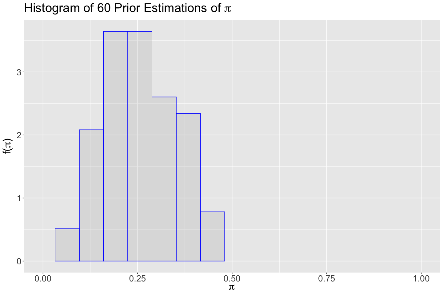
The histogram is right-skewed (a hint on the fact that, for the Beta prior, \(a < b\)). We can also obtain the summary statistics.

round(mean(tinder_prior_pi_studies$tinder_prior_pi), 3)
round(var(tinder_prior_pi_studies$tinder_prior_pi), 3)
round(sd(tinder_prior_pi_studies$tinder_prior_pi), 3)

0.255

0.01

0.098

Using the function summarize_beta_binomial(), let us obtain the theoretical values for \(\text{Beta(a = 4, b = 12)}\).

summarize_beta_binomial(a = 4, b = 12)

Warning message in summarize_beta_binomial(a = 4, b = 12):
“To summarize the posterior, 
            specify data y and n”

A data.frame: 1 × 7

model	alpha	beta	mean	mode	var	sd
<chr>	<dbl>	<dbl>	<dbl>	<dbl>	<dbl>	<dbl>
prior	4	12	0.25	0.2142857	0.01102941	0.105021

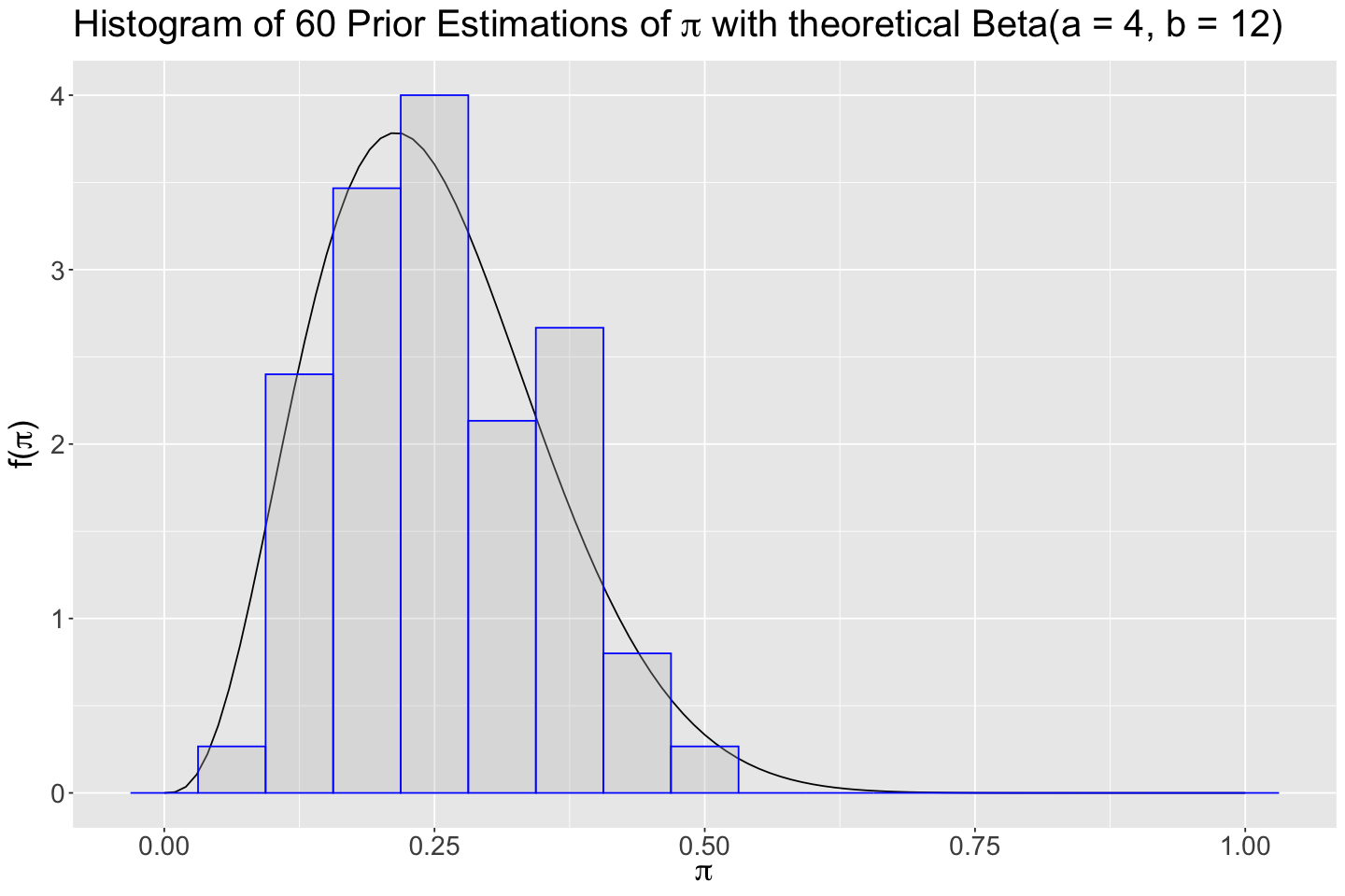
The summary statistics from tinder_prior_pi_studies are close to the theoretical prior metrics for \(\text{Beta(a = 4, b = 12)}\). Hence, let us proceed with a Beta prior with hyperparameters \(a = 4\) and \(b = 12\).

Caution

Note this might not be the only choice. Given the right-skewness in the histogram of previous studies, we could select a different pair of hyperparameters as long as \(a < b\) for our chosen theoretical Beta prior (a frequentist goodness of fit test might be an appealing option too!).

Attention

Note that the histogram below has 8 bars for better visualization.

hist_prior <- plot_beta(4, 12) +
  geom_histogram(
    data = tinder_prior_pi_studies,
    aes(x = tinder_prior_pi, y = after_stat(density)), fill = "grey", color = "blue", bins = 17, alpha = 0.3
  ) +
  ggtitle(expression(paste("Histogram of 60 Prior Estimations of ", pi, " with theoretical Beta(a = 4, b = 12)"))) +
  labs(y = expression(paste("f(", pi, ")")), x = expression(pi)) +
  theme(
    plot.title = element_text(size = 24, face = "bold"),
    axis.text = element_text(size = 17),
    axis.title = element_text(size = 21)
  )
hist_prior

We decided to use this prior:

\[\pi \sim \text{Beta}(a = 4, b = 12).\]

2.2. The Likelihood

We ran our Tinder study in Vancouver with \(n = 200\) subjects, all of them used Tinder. At the end of the study, 20 of them ended up partnered by using Tinder.

The Beta-Binomial model is set up as follows:

\[X_i \sim \text{Bernoulli}(\pi) \quad \text{with ending up partnered as success}\]

\[Y = \sum_{i = 1}^n X_i\]

\[\begin{split}\begin{gather*} Y \mid \pi \sim \text{Binomial}(n = 200, \pi) \\ \pi \sim \text{Beta}(a = 4, b = 12). \end{gather*}\end{split}\]

2.3. The Posterior

We previously derived the exact Beta posterior for \(\pi\) with the Beta-Binomial model:

\[\pi \mid Y = y \sim \text{Beta}(a' = a + y, b' = b + n - y).\]

Since \(a = 4\), \(b = 12\), \(n = 200\), and \(y = 20\); then we have:

\[\pi \mid Y = y \sim \text{Beta}(a' = 24, b' = 192).\]

Now, we can get the theoretical prior and posterior metrics.

summarize_beta_binomial(a = 4, b = 12, y = 20, n = 200)

A data.frame: 2 × 7

model	alpha	beta	mean	mode	var	sd
<chr>	<dbl>	<dbl>	<dbl>	<dbl>	<dbl>	<dbl>
prior	4	12	0.2500000	0.2142857	0.0110294118	0.10502101
posterior	24	192	0.1111111	0.1074766	0.0004551402	0.02133402

Finally, we plot the prior, likelihood, and posterior.

plot_comparison <- plot_beta_binomial(a = 4, b = 12, y = 20, n = 200) +
  labs(y = "Density", x = expression(pi)) +
  ggtitle("Comparison of Prior, Likelihood, and Posterior") +
  theme(
    plot.title = element_text(size = 24, face = "bold"),
    axis.text = element_text(size = 17),
    axis.title = element_text(size = 21),
    legend.text = element_text(size = 21, margin = margin(r = 1, unit = "cm")),
  )

plot_comparison

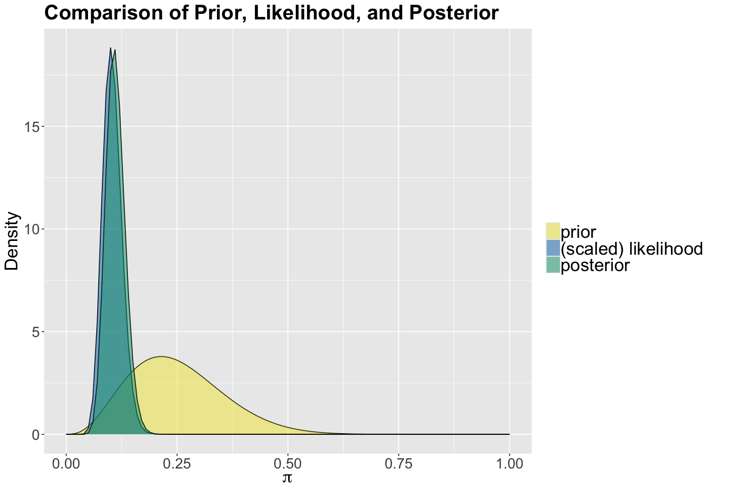
We updated our prior information, along with our own evidence, to get our Beta posterior. Note the small variability associated to the posterior \(\pi\) (less uncertainty!).

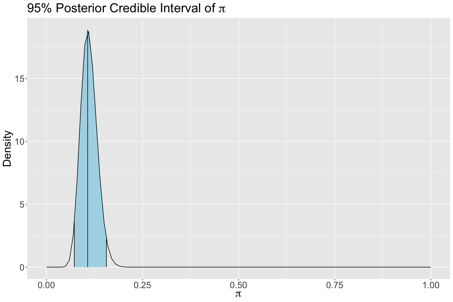
Let us obtain a 95% posterior credible interval for \(\pi\).

round(qbeta(c(0.025, 0.975), 24, 192), 2)

1. 0.07
2. 0.16

We can also plot this posterior 95% credible interval via plot_beta_ci() from bayesrules.

posterior_CI <- plot_beta_ci(24, 192, ci_level = 0.95) +
  ggtitle(expression(paste("95% Posterior Credible Interval of ", pi))) +
  labs(y = "Density", x = expression(pi)) +
  theme(
    plot.title = element_text(size = 24),
    axis.text = element_text(size = 17),
    axis.title = element_text(size = 21)
  )
posterior_CI

3. Bayesian Hypothesis Testing

3.1. One-Sided Test

We have not interpreted our posterior results yet! We could do so via the 95% posterior credible interval. Nonetheless, we will try a different approach to make inference by using our theoretical Beta posterior. For example, suppose another researcher claims the following:

In any city like Vancouver, more than 15% of the single people who use the Tinder app will eventually find a partner.

We could assess this statement by using our Bayesian results!

How do we do it? Bayesian hypothesis testing comes to the rescue. As in the case of frequentist statistics, we will have two hypotheses for \(\pi\): null \((H_0)\) and alternative \((H_a)\).

\[H_0: \pi \leq 0.15\]

\[H_a: \pi > 0.15.\]

The alternative hypothesis is associated with the researcher’s claim, whereas the null will be the opposite.

Here comes the Bayesian twist. Unlike frequentist statistics, each hypothesis will have a probability associated with the previously obtained Beta posterior. So, how do we get these probabilities? We can simply use pbeta(). Moreover, let us plot these probabilities for a better understanding.

Important

Recall the Beta posterior of \(\pi\) is a probability over probabilities.

Let \(f(\pi \mid y = 20)\) be the posterior \(\text{Beta}(a' = 24, b' = 192)\) probability density function (PDF).

Firstly, for

\[H_0: \pi \leq 0.15;\]

its posterior probability will be given by:

\[P(\pi \leq 0.15 \mid Y = 20) = \int_{0}^{0.15} f(\pi \mid y = 20) \,d\pi = 0.957.\]

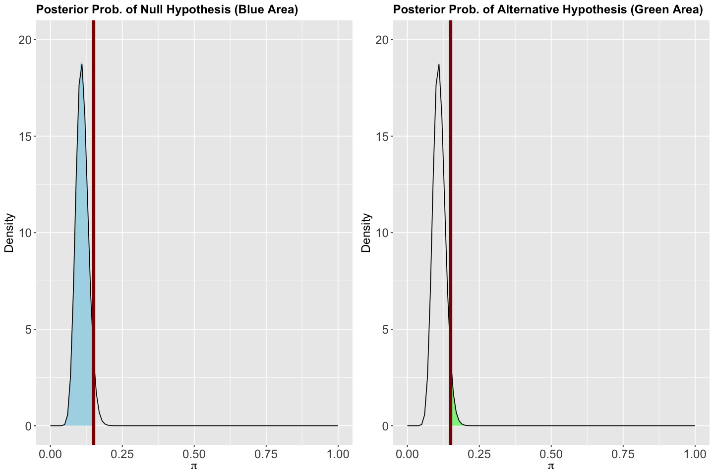
posterior_prob_H_0 <- pbeta(0.15, 24, 192)
round(posterior_prob_H_0, 3)

0.957

Now, for the alternative

\[H_a: \pi > 0.15;\]

its posterior probability will be given by:

\[P(\pi > 0.15 \mid Y = 20) = \int_{0.15}^{1} f(\pi \mid y = 20) \,d\pi = 0.043.\]

posterior_prob_H_a <- pbeta(0.15, 24, 192, lower.tail = FALSE)
round(posterior_prob_H_a, 3)

0.043

Therefore, the associated posterior probability to \(H_0\) is 0.957 and 0.043 for \(H_a\) (the complement!). The plots for the Beta posterior show these areas. Note a vertical red line crosses \(\pi = 0.15\) on the \(x\)-axes.

# Modified code, from bayesrules, to plot the posterior probabilities of H_0 and H_a.

plot_posterior_prob_H_0 <- ggplot(data.frame(x = c(0, 1)), aes(x = x)) +
  stat_function(
    fun = dbeta,
    args = list(24, 192),
    xlim = c(0, 0.15),
    geom = "area",
    fill = "lightblue"
  ) +
  stat_function(
    fun = dbeta,
    args = list(24, 192)
  ) +
  geom_vline(xintercept = 0.15, colour = "darkred", linewidth = 2) +
  ggtitle("Posterior Prob. of Null Hypothesis (Blue Area)") +
  labs(y = "Density", x = expression(pi)) +
  theme(
    plot.title = element_text(size = 14.5, face = "bold"),
    axis.text = element_text(size = 14.5),
    axis.title = element_text(size = 14.5)
  ) +
  xlim(0, 1) +
  ylim(0, 20)

plot_posterior_prob_H_a <- ggplot(data.frame(x = c(0, 1)), aes(x = x)) +
  stat_function(
    fun = dbeta,
    args = list(24, 192),
    xlim = c(0.15, 1),
    geom = "area",
    fill = "lightgreen"
  ) +
  stat_function(
    fun = dbeta,
    args = list(24, 192)
  ) +
  geom_vline(xintercept = 0.15, colour = "darkred", linewidth = 2) +
  ggtitle("Posterior Prob. of Alternative Hypothesis (Green Area)") +
  labs(y = "Density", x = expression(pi)) +
  theme(
    plot.title = element_text(size = 14.5, face = "bold"),
    axis.text = element_text(size = 14.5),
    axis.title = element_text(size = 14.5)
  ) +
  xlim(0, 1) +
  ylim(0, 20)

plot_grid(plot_posterior_prob_H_0, plot_posterior_prob_H_a)

Summarizing, we have two posterior probabilities:

\[P(H_0 \mid Y = 20) = P(\pi \leq 0.15 \mid Y = 20) = 0.957\]

\[P(H_a \mid Y = 20) = P(\pi > 0.15 \mid Y = 20) = 0.043.\]

Now, we can compute the posterior odds that \(\pi > 0.15\):

\[\text{posterior odds} = \frac{P(H_a \mid Y = 20)}{P(H_0 \mid Y = 20)} = \frac{0.043}{0.957} = 0.045.\]

posterior_odds <- posterior_prob_H_a / posterior_prob_H_0
round(posterior_odds, 3)

0.045

How can we interpret this ratio? We can state that \(\pi\) is 22.22 times \(\big(\frac{1}{0.045}\big)\) more likely to be less or equal than 0.15 compared to being above 0.15 using our posterior model.

In Bayesian hypothesis testing, we do not use \(p\)-values. However, there is an analogous metric called the Bayes factor. This factor will compare the posterior odds versus the prior odds. It will shed light on how our inference on \(\pi\) changed given our observed evidence (reflected in the posterior distribution via the Bayes’ rule).

We already computed the posterior odds, let us proceed with the prior odds. Let \(f(\pi)\) be the prior \(\text{Beta}(a = 4, b = 12)\) PDF.

For

\[H_0: \pi \leq 0.15;\]

its prior probability will be given by:

\[P(\pi \leq 0.15) = \int_{0}^{0.15} f(\pi) \,d\pi = 0.177.\]

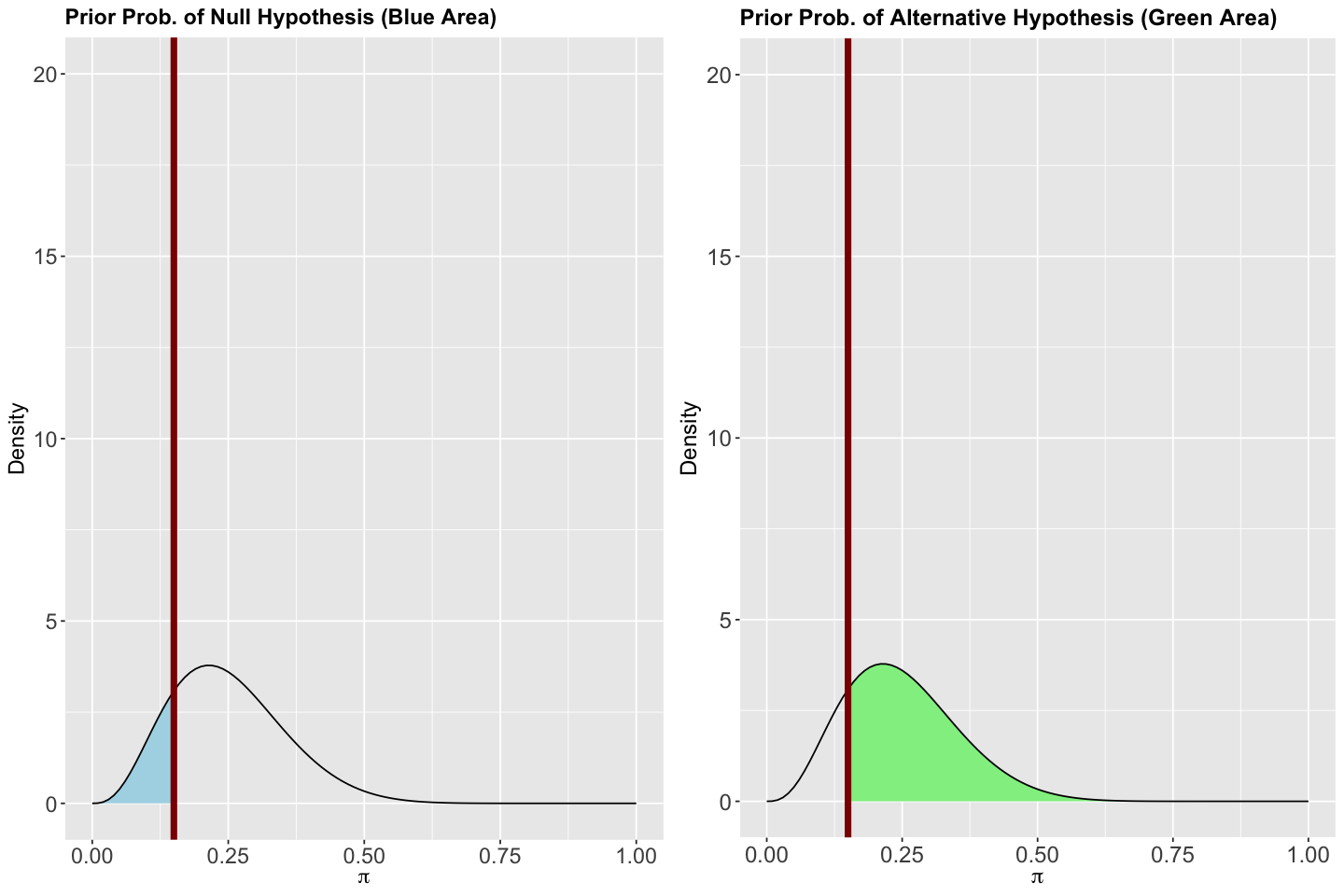
prior_prob_H_0 <- pbeta(0.15, 4, 12)
round(prior_prob_H_0, 3)

0.177

Now, for the alternative

\[H_a: \pi > 0.15;\]

its prior probability will be given by:

\[P(\pi > 0.15) = \int_{0.15}^{1} f(\pi) \,d\pi = 0.823.\]

prior_prob_H_a <- pbeta(0.15, 4, 12, lower.tail = FALSE)
round(prior_prob_H_a, 3)

0.823

Thus, the associated prior probability to \(H_0\) is 0.177 and 0.823 for \(H_a\) (the complement!). The plots for the Beta prior show these areas. Note a vertical red line crosses \(\pi = 0.15\) on the \(x\)-axes.

# Modified code, from bayesrules, to plot the posterior probabilities of H_0 and H_a.

plot_prior_prob_H_0 <- ggplot(data.frame(x = c(0, 1)), aes(x = x)) +
  stat_function(
    fun = dbeta,
    args = list(4, 12),
    xlim = c(0, 0.15),
    geom = "area",
    fill = "lightblue"
  ) +
  stat_function(
    fun = dbeta,
    args = list(4, 12)
  ) +
  geom_vline(xintercept = 0.15, colour = "darkred", linewidth = 2) +
  ggtitle("Prior Prob. of Null Hypothesis (Blue Area)") +
  labs(y = "Density", x = expression(pi)) +
  theme(
    plot.title = element_text(size = 14, face = "bold"),
    axis.text = element_text(size = 14),
    axis.title = element_text(size = 14)
  ) +
  xlim(0, 1) +
  ylim(0, 20)

plot_prior_prob_H_a <- ggplot(data.frame(x = c(0, 1)), aes(x = x)) +
  stat_function(
    fun = dbeta,
    args = list(4, 12),
    xlim = c(0.15, 1),
    geom = "area",
    fill = "lightgreen"
  ) +
  stat_function(
    fun = dbeta,
    args = list(4, 12)
  ) +
  geom_vline(xintercept = 0.15, colour = "darkred", linewidth = 2) +
  ggtitle("Prior Prob. of Alternative Hypothesis (Green Area)") +
  labs(y = "Density", x = expression(pi)) +
  theme(
    plot.title = element_text(size = 14.5, face = "bold"),
    axis.text = element_text(size = 14.5),
    axis.title = element_text(size = 14.5)
  ) +
  xlim(0, 1) +
  ylim(0, 20)

plot_grid(plot_prior_prob_H_0, plot_prior_prob_H_a)

Summarizing, we have two prior probabilities:

\[P(H_0) = P(\pi \leq 0.15) = 0.177\]

\[P(H_a) = P(\pi > 0.15) = 0.823.\]

We can compute the prior odds that \(\pi > 0.15\):

\[\text{prior odds} = \frac{P(H_a)}{P(H_0)} = \frac{0.823}{0.177} = 4.639.\]

prior_odds <- prior_prob_H_a / prior_prob_H_0
round(prior_odds, 3)

4.639

How can we interpret this ratio? We can state that \(\pi\) is 4.639 times more likely to be above 0.15 compared to being less or equal than 0.15 using our prior model.

The Bayes factor is computed as follows:

\[\text{Bayes Factor} = \frac{\text{posterior odds}}{\text{prior odds}} = 0.01.\]

bayes_factor <- posterior_odds / prior_odds
round(bayes_factor, 2)

0.01

How can we interpret the Bayes factor?

In general, there are three possible scenarios:

• \(\text{Bayes Factor} = 1\): The plausibility of \(H_a\) remained the same, even though we collected new evidence (our study) and applied the Bayes’ rule.

• \(\text{Bayes Factor} > 1\): The plausibility of \(H_a\) increased once we have collected more evidence (our study) and applied the Bayes’ rule.

• \(\text{Bayes Factor} < 1\): The plausibility of \(H_a\) decreased once we have collected more evidence (our study) and applied the Bayes’ rule.

Therefore, the researcher’s statement is less plausible in the light of our own evidence!

Exercise 16

Suppose you want to apply the previous hypothesis testing procedure using the approximate posterior samples from MCMC. Hence, there is no analytical solution to the corresponding integrals to obtain the probabilities associated with the posterior odds. Actually, we do not even have an exact PDF to integrate!

What workaround can you use in that regard to obtain the posterior odds?

3.2. Two-Sided Test

Now let us suppose the researcher only wants to assess whether or not 15% of the single people who use the Tinder app will eventually find a partner (in any city like Vancouver). This is a two-sided test:

\[H_0: \pi = 0.15\]

\[H_a: \pi \neq 0.15.\]

However, in a continuous parameter like \(\pi\), there is a problem:

\[P(\pi = 0.15 \mid Y = 20) = \int_{0.15}^{0.15} f(\pi \mid y = 20) \,d\pi = 0.\]

We cannot obtain the posterior odds! And forget about the prior odds (it is the same problem).

There is a tweak to solve this two-sided test, we can restate our hypotheses as some range of plausible values (\(\pm 0.10\), for instance):

\[H_0: \pi \in (0.05, 0.25)\]

\[H_a: \pi \notin (0.05, 0.25).\]

And let us use our 95% posterior credible interval to evaluate this test:

round(qbeta(c(0.025, 0.975), 24, 192), 2)

1. 0.07
2. 0.16

This credible interval falls within the hypothesized range in \(H_0\). Therefore, we have reasonable posterior evidence in favour of \(H_0\) with 95% probability!

4. Wrapping Up

• We can extend the Bayesian paradigm to a regression framework where the systematic component will become part of our likelihood.

• The use of priors on our regression parameters of interest allows us to make more clever modelling (i.e., choosing the right support for our parameters). Nonetheless, obtaining prior knowledge can be a challenging task.

• Stan is a powerful tool that will even allow us to estimate non-linear regression models using MCMC. Moreover, the algorithm is the same for all the regression approaches!

• Bayesian hypothesis testing has a framework for assigning probabilities to our hypotheses based on our prior and posterior models.

• The Bayes Factor is the substitute to \(p\)-value in hypothesis testing.