Lecture 1 - Multiple Comparisons#
High-Level Goals of this Course#
Distinguish between experimentally-generated data and observational data, with particular reference to the strength of ensuing statistical conclusions regarding causality.
Fit and interpret regression models for observational data, with particular reference to adjustment for potential confounding variables.
Apply the principle of “block what you can, randomize what you cannot” in designing an A/B testing experiments.
Firstly, let us make a block overview!#
Lecture 1: Multiple comparisons and false discovery (“Can I believe in science?”).
Lecture 2: Confounding, randomized versus non-randomized studies (“Okay, it’s not so bad…”).
Lectures 3-5: Randomized study issues (“Okay, it’s even better than I thought…”).
Lectures 6-8: Non-randomized study issues (“It’s hopeless!”).
In this course, there will be few new statistical tools to pick up. But we will need (and perhaps hone) our regression skills!
Again, this course is entirely taught in R with a reasonable mathematical and statistical basis. There will be eight lectures and four labs. We strongly recommend reviewing the following frequentist courses:
DSCI 551: Descriptive Statistics and Probability for Data Science for basic statistical and probabilistic concepts, and familiarity with the mathematical notation
DSCI 552 - Statistical Inference and Computation I for statistical inference concepts with a frequentist approach.
DSCI 561 - Regression I for ordinary least-squares (OLS)
DSCI 562 - Regression II for more advanced regression models.
Attention
Keep in mind the following: this is a concepts block.
What is the Relevance of this Course to Data Science?#
Indirect Relevance#
This course is an inherent part of your statistical training given your current statistical maturity. You already learned a comprehensive set of statistical tools in the previous courses.
Moreover, we will stress the concept of “joined-up thinking” on the entire data pipeline:
How data are collected.
How data are analyzed.
How conclusions are drawn.
The strength of the resulting story (i.e., how robust the data story-telling is).
Important
This “joined-up thinking” is related to the Data Science Workflow from DSCI 562 - Regression II.
Direct Relevance#
Throughout the block, we will review the following two major classes of statistical studies to adress causality:
Randomized studies: In this class of studies, the researcher can randomly allocate the subjects to one of the experimental treatments. An experimental treatment is a given testing strategy (e.g., in pharmaceutical trials, a placebo is a control treatment whereas the experimental drug is the treatment of interest). Specifically, in Data Science, we could encounter the example below.
Example
A/B testing for website optimization:
Does a tweak to a website improve user experience and/or generate more sales? (i.e., control website A versus experimental website B).
Can we end a test early? This is called early-stopping in statistical jargon.
Non-randomized studies: In many different case studies, treatment randomization is impossible. Hence, we need to apply certain statistical concepts and tools to address our specific inquiries.
Example
Pharmaco-epidemiology problems and electronic health records:
We might encounter different data pipelines for massive healthcare utilization databases to obtain knowledge about drug efficacy and safety.
Today’s Learning Objectives#
Review frequentist hypothesis testing.
Examine the misuse of \(p\)-values in scientific literature.
Demonstrate the misuse of \(p\)-values via a simulation.
Explain the macro-properties of carrying out many hypothesis tests in the context of a single dataset.
Use Bonferroni and False Discovery Rate correction to alter the macro-properties when conducting many hypothesis tests.
Contrast the Bonferroni correction with the False Discovery Rate.
Loading R Packages#
options(repr.matrix.max.rows = 8, repr.matrix.max.cols = 7)
library(mvtnorm)
library(ggplot2)
library(reshape2)
library(tidyverse)
1. Hypothesis Testing Review#
In statistical inference, we have two hypotheses: the null \(H_0\) and the alternative \(H_a\).
\(H_0\) represents the status quo in our case study, whereas \(H_a\) represents our hypothesis of interest. Furthermore, recall there are two types of errors shown in the table below.
\(H_0\) is true |
\(H_0\) is not true |
|
|---|---|---|
Fail to reject \(H_0\) |
Correct (TRUE NEGATIVE) |
Type II Error (FALSE NEGATIVE) |
Reject \(H_0\) |
Type I Error (FALSE POSITIVE) |
Correct (TRUE POSITIVE) |
These errors are I (false positive) and II (false negative). Their setup is targeted towards rejecting or not rejecting \(H_0\), given that \(H_0\) is true or not. Moreover, these errors are measured in probabilities.
The frequentist hypothesis testing process is the following:
We need to set up a pre-specified significance level (usually \(\alpha = 0.05\)). The significance level \(\alpha\) will be our tolerance to type I error: rejecting the null hypothesis when in fact is true.
Compute a test statistic from our sampled data. This test statistic will have a sampling distribution under \(H_0\).
Compare the test statistic against a certain quantile threshold under \(H_0\), then:
Reject \(H_0\) in favour of \(H_a\) if the test statistic exceeds this quantile threshold under \(H_0\).
Do not reject \(H_0\) otherwise.
Attention
The quantile threshold is chosen such that
1.1. \(p\)-value#
An alternative way of performing Step 3 is computing the \(p\)-value associated to the test statistic under \(H_0\).
Let us start with some mathematical notation. For this Step 3, in general let the test statistic be \(T\) (note the random variable notation as an uppercase!) and the quantile threshold \(c_\alpha\). Thus, we would reject \(H_0\) if
Now, for our observed data, the test statistic will be \(t_{\text{obs}}\) (note the lowercase notation!). In probability notation, the \(p\)-value can be represented as:
Attention
The \(p\)-value is the chance of getting a test statistic as or more extreme than what you actually got as observed data, presuming \(H_0\) is true. We will reject \(H_0\) if
1.2. Graphical Overview of the Hypothesis Testing#
All the previous process can also be put as in the diagram below.
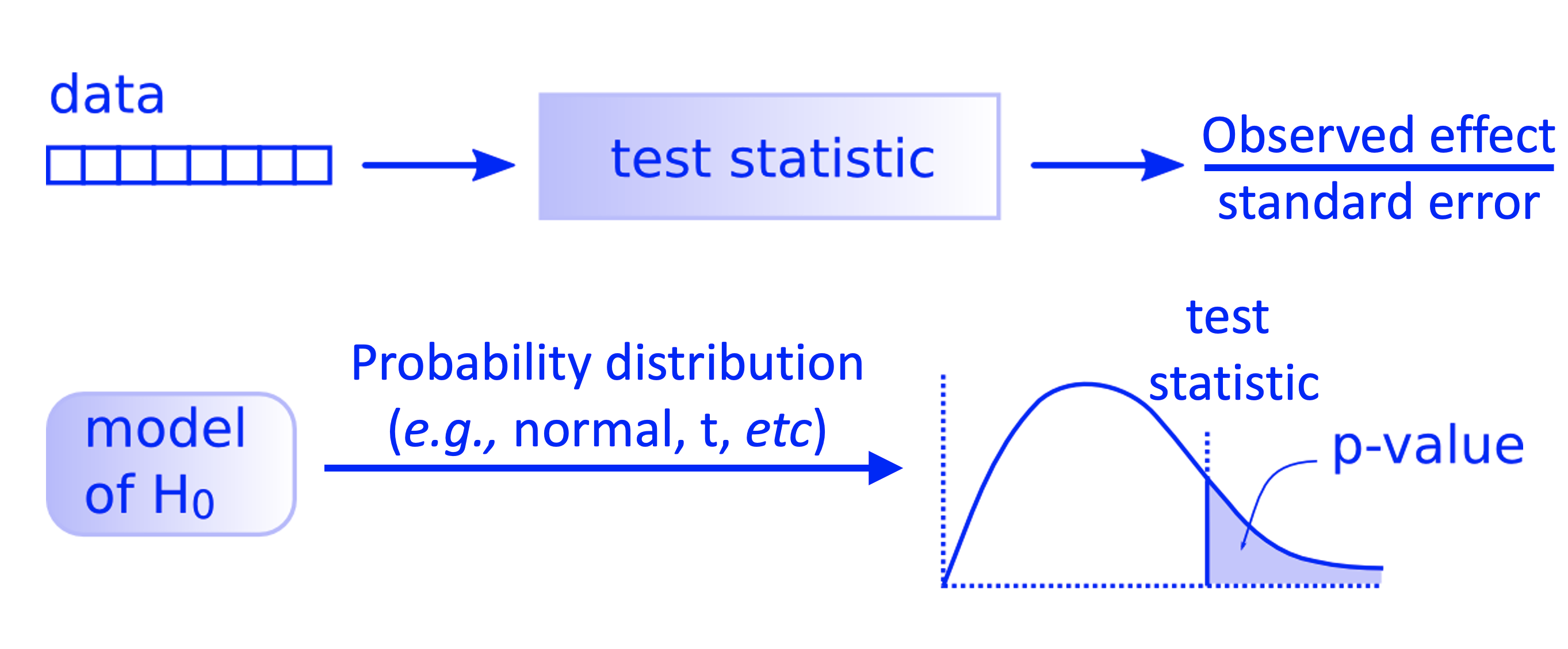
Fig. 1 Workflow of a theory-based hypothesis testing.#
1.3. Testing Procedure in a Nutshell#
Let us start with some coding. The significance level \(\alpha = 0.05\) testing procedure can be cast as:
Reject \(H_0\) if \(p\text{-value} < \alpha = 0.05\).
Do not reject \(H_0\) otherwise.
This process can be coded as in the function below.
hypothesis.test <- function(alpha = 0.05, p_value) {
  reject <- (p_value < alpha)
  return(reject)
}
2. Hypothesis Testing in Science#
It is well known that it is easier to publish your work in a better journal if you have one (or more!) statistically significant findings at the (conventional) \(\alpha = 0.05\) level.
2.1. Why does that happen?#
This is in the function of what the scientific community considers as “interesting results”:
By construction, the null hypothesis is “conservative”/”boring”/”status quo.”
The alternative hypothesis is usually more interesting than the null hypothesis, e.g., eating chocolate and living longer are associated. So a \(p\text{-value} < 0.05\) is exciting!
2.2. When \(p\text{-value} > 0.05\)#
We have to make a controversial statement: obtaining \(p\text{-value} > 0.05\) is ambiguous!
Why are we stating that? Here are some reasons:
Data did not provide strong evidence against the null hypothesis.
Maybe our test has low power.
Therefore, the New York Times (for instance) is not putting that in the Science section. For instance, THESE HEADLINES WILL NEVER HAPPEN:
“Scientists conclude that they do not have enough data.”
“Null hypothesis not rejected.”
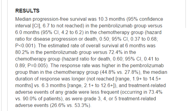
2.3. An Journal Example on Statistical Significant Results#
We often see reports of small \(p\)-values in abstracts of scientific papers. This is an example:

3. An Inconvenient Truth#
It seems that this standard scientific practice of rejecting the null hypothesis \(H_0\) when the \(p\text{-value} < 0.05\) is a good one. Nevertheless, carrying out many comparisons (tests) in a single dataset but then only mentioning those that produce \(p\text{-value} < 0.05\) is cheating!
We discussed this matter in DSCI 552 and is called \(p\)-hacking:
We have to avoid a practice known as \(p\)-hacking in which we perform many different tests on our data to obtain any significant result to publish. By doing this, multiple testing occurs, which inflates our type I error if we do not control it with some available correction (e.g., Bonferroni correction).
Keep in mind one important concept here: Bonferroni correction. It will be critical in this lecture.
3.1. Our First Simulation#
Throughout the course, we will run different simulations to make key proofs of concept. We will start with the inflation of the type I error. Hence, let us run a simulation in three steps.
Step 1: Setting our 400 random alternative hypotheses#
Suppose I want to test \(20 \times 20\) food-health associations (i.e., 400 hypothesis testings based on 400 regression models on a single dataset).
# 20 food and health variables
nvars <- 20
# Food and human body parts
foods <- c(
  "Peanuts", "Dark Chocolate", "Wine", "Grass", "Cinnamon",
  "Ice Cream", "Potatoes", "Doritos", "Salsa", "Bugs",
  "Soap", "Yogurt", "Gatorade", "Milk Chocolate", "Raisins",
  "Cured Meat", "Raw Fish", "Dirt", "Toothpaste", "Apples"
)
health <- c(
  "heart", "lung", "gut", "cognitive", "foot",
  "arm", "eye", "hair", "dental", "ear",
  "knee", "hip", "fingernail", "joint", "shoulder",
  "muscle", "eyelash", "kidney", "skin", "mental"
)
# Class of association
outcome <- c("good","bad")
Once we have our possible variables and outcomes, let us build our 400 alternative hypotheses. We will do this randomly for outcome.
set.seed(554)
# Grid of all possible pairs
experiments <- expand.grid(foods, health)
names(experiments)[1:2] <- c("food", "health")
# The random outcomes associated to our 400 alternative hypothesis!
experiments$outcome <- outcome[sample.int(2, nvars * nvars, replace = TRUE)]
experiments
| food | health | outcome |
|---|---|---|
| <fct> | <fct> | <chr> |
| Peanuts | heart | good |
| Dark Chocolate | heart | bad |
| Wine | heart | bad |
| Grass | heart | bad |
| ⋮ | ⋮ | ⋮ |
| Raw Fish | mental | bad |
| Dirt | mental | good |
| Toothpaste | mental | bad |
| Apples | mental | bad |
Then, we build our 400 alternative hypotheses.
alternative_hypotheses <- paste("Eating ", tolower(experiments$food),
  " is ", experiments$outcome,
  " for ", experiments$health, " health.",
  sep = ""
)
as.data.frame(alternative_hypotheses)
| alternative_hypotheses |
|---|
| <chr> |
| Eating peanuts is good for heart health. |
| Eating dark chocolate is bad for heart health. |
| Eating wine is bad for heart health. |
| Eating grass is bad for heart health. |
| ⋮ |
| Eating raw fish is bad for mental health. |
| Eating dirt is good for mental health. |
| Eating toothpaste is bad for mental health. |
| Eating apples is bad for mental health. |
Step 2: Generating our Simulated Dataset#
It is time to generate our simulated dataset to test our 400 alternative hypotheses. This dataset will be comprised of 20 continuous \(X\) variables (regressors) and 20 \(Y\) continuous variables (responses) measured on each of \(n = 500\) people. Therefore:
\(X\) variables are a person’s intake of different foods.
\(Y\) variables are different measures of a person’s health.
We will need to use a made-up function simulate_p() to run our simulation. This simulation will include 400 simple regression models and record their corresponding \(p\)-values to assess the statistical association between each \(X\) and \(Y\). Note, we will generate our random data so that none of the \(X\) variables are associated with any of the \(Y\) variables (i.e., \(H_0\) is in fact true!). Each one of the 400 generic null hypotheses is set up as:
Attention
Below is the R code to generate the random numbers in function simulate_p(). Reviewing this code is out of the scope of this lecture since it involves Multivariate Normal concepts. As optional practice, feel free to go through this code (you will find some useful comments on the way).
Show code cell source
simulate_p <- function(nvars, nobs, rho) {
  sigmas_sq <- (1 - rho) * diag(nvars) # We assign the same variance to all nvars
    # (main diagonal in an nvar times nvar variance-covariance matrix)
  if (nvars > 1) { # Now, we assign the same pairwise covariances in
      # the nvar times nvar variance-covariance matrix
      # (SO ANY VARIABLE WILL NOT STAND OUT AS STATISTICALLY SIGNIFICANT!)
    sigmas_sq <- sigmas_sq + rho * matrix(1, nvars, nvars)
  }
  x <- rmvnorm( # We generate nobs times nvar multivariate normal random numbers (regressors)
      # with vector mean of zeros and variance-covariance matrix sigmas_sq
    n = nobs, mean = rep(0, nvars),
    sigma = sigmas_sq
  )
  y <- rmvnorm( # We generate nobs times nvar multivariate normal random numbers (responses)
      # with vector mean of zeros and variance-covariance matrix sigmas_sq
    n = nobs, mean = rep(0, nvars),
    sigma = sigmas_sq
  )

  # Finallly, we run nvar times nvar simple linear regressions of each X versus each Y
  # Then, we record the p-value from our lm() summaries
  pmat <- matrix(NA, nvars, nvars)
  for (i in 1:nvars) {
    for (j in 1:nvars) {
      pmat[i, j] <- anova(lm(y[, i] ~ x[, j]))$Pr[1]
    }
  }
  return(pmat) # pmat is the nvar x nvar matrix of p-values
}
Step 3: Running the 400 Regression Models#
Then, we run all 400 regressions of one of the \(Y\)’s on one of the \(X\)’s.
sig_alpha <- 0.05 # alpha threshold
nvars <- 20
nobs <- 500
rho <- 0.75 # Variance-covariance matrix parameter denoting the same pairwise covariance for all the nvars, i.e.,
# the same status quo

set.seed(12345) # Global reproducibility
pval <- simulate_p(nvars, nobs, rho)
3.2. Checking our Simulation Results#
We will check how many \(p\)-values are below sig_alpha in pval (i.e., how many times we committed type I error).
162 pairwise comparisons, out of 400 (i.e., 40.5%), are rejecting \(H_0\) when in fact is true!
sum(pval < sig_alpha)
options(repr.plot.height = 8, repr.plot.width = 14)

p.val.hist <- pval %>%
  melt() %>%
  ggplot(aes(x = value)) +
  geom_histogram(binwidth = 0.025, aes(y = after_stat(count)), colour = "black", fill = "gray") +
  geom_vline(aes(xintercept = sig_alpha), color = "blue", linetype = "dashed", linewidth = 1) +
  xlab("p-values") +
  theme(
    plot.title = element_text(size = 18, face = "bold"),
    axis.text = element_text(size = 17),
    axis.title = element_text(size = 18),
    legend.position = "none"
  ) +
  ggtitle("Histogram of Relative Frequencies of p-values Coming from 400 Simple Regression Models")
p.val.hist
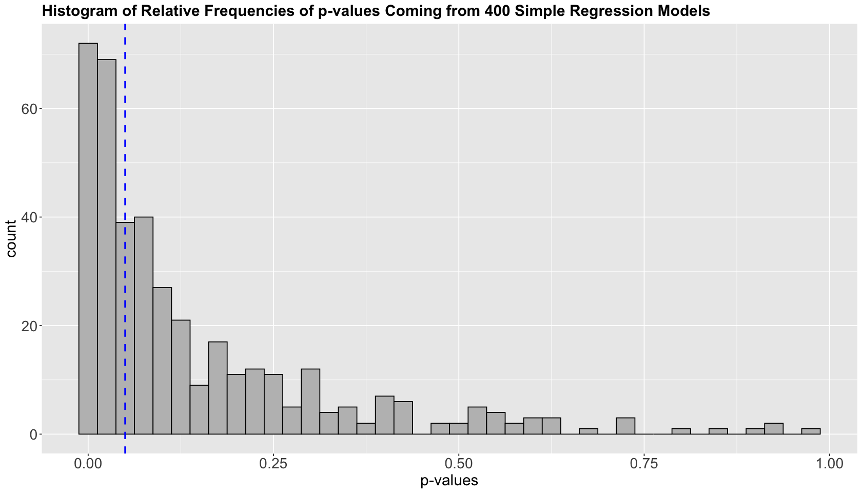
The histogram above plots the \(p\)-values on the \(x\)-axis as counts on the \(y\) axis. The vertical dashed blue line indicates the \(\alpha\) threshold.
Imagine the \(p\)-values in the matrix pval correspond to the alternative hypotheses we constructed in alternative_hypotheses. Therefore, we can publish 162 papers, each generating a headline:
melt_p <- melt(pval) # Melting matrix pval before filtering those spurious significant results
melt_p
| Var1 | Var2 | value |
|---|---|---|
| <int> | <int> | <dbl> |
| 1 | 1 | 0.01144746 |
| 2 | 1 | 0.02435357 |
| 3 | 1 | 0.03857421 |
| 4 | 1 | 0.54722977 |
| ⋮ | ⋮ | ⋮ |
| 17 | 20 | 0.08290290 |
| 18 | 20 | 0.16151143 |
| 19 | 20 | 0.07920598 |
| 20 | 20 | 0.40985565 |
# Now, we filter those spurious significant results and their corresponding alternative hypotheses
print(alternative_hypotheses[melt_p$value < sig_alpha])
  [1] "Eating peanuts is good for heart health."
  [2] "Eating dark chocolate is bad for heart health."
  [3] "Eating wine is bad for heart health."
  [4] "Eating bugs is good for heart health."
  [5] "Eating peanuts is good for lung health."
  [6] "Eating dark chocolate is good for lung health."
  [7] "Eating wine is good for lung health."
  [8] "Eating bugs is good for lung health."
  [9] "Eating dark chocolate is bad for gut health."
 [10] "Eating wine is good for gut health."
 [11] "Eating bugs is good for gut health."
 [12] "Eating toothpaste is bad for gut health."
 [13] "Eating wine is good for cognitive health."
 [14] "Eating peanuts is good for foot health."
 [15] "Eating dark chocolate is bad for foot health."
 [16] "Eating wine is bad for foot health."
 [17] "Eating cinnamon is bad for foot health."
 [18] "Eating ice cream is good for foot health."
 [19] "Eating potatoes is good for foot health."
 [20] "Eating doritos is bad for foot health."
 [21] "Eating salsa is good for foot health."
 [22] "Eating bugs is bad for foot health."
 [23] "Eating soap is bad for foot health."
 [24] "Eating yogurt is bad for foot health."
 [25] "Eating gatorade is good for foot health."
 [26] "Eating milk chocolate is good for foot health."
 [27] "Eating raisins is good for foot health."
 [28] "Eating cured meat is bad for foot health."
 [29] "Eating raw fish is good for foot health."
 [30] "Eating dirt is good for foot health."
 [31] "Eating toothpaste is good for foot health."
 [32] "Eating apples is good for foot health."
 [33] "Eating peanuts is bad for arm health."
 [34] "Eating dark chocolate is good for arm health."
 [35] "Eating wine is bad for arm health."
 [36] "Eating grass is bad for arm health."
 [37] "Eating cinnamon is good for arm health."
 [38] "Eating ice cream is bad for arm health."
 [39] "Eating potatoes is good for arm health."
 [40] "Eating doritos is bad for arm health."
 [41] "Eating salsa is good for arm health."
 [42] "Eating bugs is bad for arm health."
 [43] "Eating soap is good for arm health."
 [44] "Eating yogurt is bad for arm health."
 [45] "Eating milk chocolate is good for arm health."
 [46] "Eating raisins is bad for arm health."
 [47] "Eating cured meat is good for arm health."
 [48] "Eating raw fish is good for arm health."
 [49] "Eating dirt is good for arm health."
 [50] "Eating toothpaste is good for arm health."
 [51] "Eating apples is good for arm health."
 [52] "Eating dark chocolate is bad for eye health."
 [53] "Eating wine is good for eye health."
 [54] "Eating bugs is good for eye health."
 [55] "Eating soap is good for eye health."
 [56] "Eating yogurt is bad for eye health."
 [57] "Eating toothpaste is good for eye health."
 [58] "Eating dark chocolate is bad for hair health."
 [59] "Eating wine is good for hair health."
 [60] "Eating peanuts is bad for dental health."
 [61] "Eating dark chocolate is good for dental health."
 [62] "Eating wine is good for dental health."
 [63] "Eating ice cream is bad for dental health."
 [64] "Eating potatoes is good for dental health."
 [65] "Eating doritos is good for dental health."
 [66] "Eating salsa is good for dental health."
 [67] "Eating bugs is good for dental health."
 [68] "Eating soap is bad for dental health."
 [69] "Eating yogurt is bad for dental health."
 [70] "Eating dirt is good for dental health."
 [71] "Eating toothpaste is bad for dental health."
 [72] "Eating peanuts is good for ear health."
 [73] "Eating dark chocolate is good for ear health."
 [74] "Eating wine is good for ear health."
 [75] "Eating doritos is bad for ear health."
 [76] "Eating salsa is bad for ear health."
 [77] "Eating bugs is bad for ear health."
 [78] "Eating soap is good for ear health."
 [79] "Eating peanuts is bad for knee health."
 [80] "Eating dark chocolate is good for knee health."
 [81] "Eating wine is good for knee health."
 [82] "Eating potatoes is good for knee health."
 [83] "Eating salsa is good for knee health."
 [84] "Eating bugs is good for knee health."
 [85] "Eating soap is good for knee health."
 [86] "Eating raisins is good for knee health."
 [87] "Eating raw fish is bad for knee health."
 [88] "Eating dirt is bad for knee health."
 [89] "Eating toothpaste is bad for knee health."
 [90] "Eating peanuts is good for fingernail health."
 [91] "Eating dark chocolate is bad for fingernail health."
 [92] "Eating wine is bad for fingernail health."
 [93] "Eating ice cream is bad for fingernail health."
 [94] "Eating salsa is bad for fingernail health."
 [95] "Eating bugs is good for fingernail health."
 [96] "Eating toothpaste is bad for fingernail health."
 [97] "Eating peanuts is good for joint health."
 [98] "Eating dark chocolate is bad for joint health."
 [99] "Eating wine is good for joint health."
[100] "Eating cinnamon is good for joint health."
[101] "Eating ice cream is good for joint health."
[102] "Eating potatoes is good for joint health."
[103] "Eating doritos is good for joint health."
[104] "Eating salsa is bad for joint health."
[105] "Eating bugs is good for joint health."
[106] "Eating soap is bad for joint health."
[107] "Eating yogurt is good for joint health."
[108] "Eating gatorade is good for joint health."
[109] "Eating milk chocolate is bad for joint health."
[110] "Eating raisins is good for joint health."
[111] "Eating cured meat is bad for joint health."
[112] "Eating raw fish is bad for joint health."
[113] "Eating dirt is bad for joint health."
[114] "Eating toothpaste is good for joint health."
[115] "Eating apples is bad for joint health."
[116] "Eating peanuts is good for shoulder health."
[117] "Eating dark chocolate is good for shoulder health."
[118] "Eating wine is good for shoulder health."
[119] "Eating cinnamon is bad for shoulder health."
[120] "Eating ice cream is bad for shoulder health."
[121] "Eating potatoes is bad for shoulder health."
[122] "Eating doritos is good for shoulder health."
[123] "Eating salsa is good for shoulder health."
[124] "Eating bugs is bad for shoulder health."
[125] "Eating soap is bad for shoulder health."
[126] "Eating yogurt is good for shoulder health."
[127] "Eating raisins is bad for shoulder health."
[128] "Eating raw fish is good for shoulder health."
[129] "Eating toothpaste is bad for shoulder health."
[130] "Eating peanuts is good for muscle health."
[131] "Eating dark chocolate is bad for muscle health."
[132] "Eating wine is bad for muscle health."
[133] "Eating ice cream is good for muscle health."
[134] "Eating potatoes is good for muscle health."
[135] "Eating salsa is good for muscle health."
[136] "Eating bugs is bad for muscle health."
[137] "Eating soap is good for muscle health."
[138] "Eating yogurt is bad for muscle health."
[139] "Eating raisins is bad for muscle health."
[140] "Eating raw fish is bad for muscle health."
[141] "Eating dirt is bad for muscle health."
[142] "Eating toothpaste is bad for muscle health."
[143] "Eating dark chocolate is good for eyelash health."
[144] "Eating wine is good for eyelash health."
[145] "Eating toothpaste is good for eyelash health."
[146] "Eating peanuts is bad for kidney health."
[147] "Eating dark chocolate is bad for kidney health."
[148] "Eating wine is good for kidney health."
[149] "Eating peanuts is bad for skin health."
[150] "Eating dark chocolate is bad for skin health."
[151] "Eating wine is bad for skin health."
[152] "Eating ice cream is bad for skin health."
[153] "Eating potatoes is bad for skin health."
[154] "Eating doritos is bad for skin health."
[155] "Eating salsa is bad for skin health."
[156] "Eating bugs is bad for skin health."
[157] "Eating yogurt is good for skin health."
[158] "Eating raisins is bad for skin health."
[159] "Eating cured meat is good for skin health."
[160] "Eating toothpaste is good for skin health."
[161] "Eating dark chocolate is bad for mental health."
[162] "Eating bugs is good for mental health."
But this does not make any sense! We would be publishing misleading and non-sense results!
Exercise 1
Why are we seeing so many spurious statistically significant comparisons here?
A. We are inflating our Type I error.
B. We are inflating our Type II error.
C. We are inflating both Types of error: I and II.
Exercise 2
How might we address this problem of so many spurious statistically significant comparisons?
A. Let us increase our power \(1 - \beta\).
B. Let us decrease our significance level \(\alpha\).
C. Let us decrease our significance level \(\alpha\) and increase our power \(1 - \beta\).
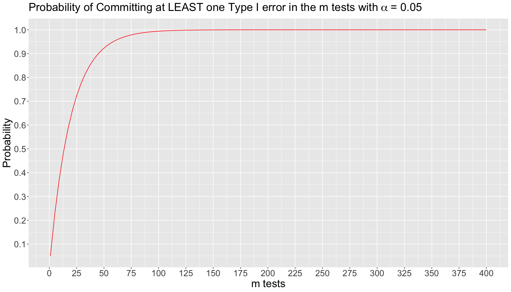
3.3. What is going on in our previous simulation?#
Suppose we run \(m\) independent tests on the same dataset. Each \(i\)th test \((i = 1, \dots m)\) has the following probability of committing Type I error:
The probability of NOT committing Type I error in the \(i\)th test is the following:
The probability of NOT committing Type I error in ALL the \(m\) tests is an intersection of complements:
Finally, the probability of committing AT LEAST one Type I error in the \(m\) tests is the complement of the previous intersection:
The inflated probability corresponds to committing AT LEAST one Type I error in the \(m\) tests. We can plot this theoretical behaviour by varying \(m\) on the \(x\)-axis as follows:
Show code cell source
x <- 1:400
df <- data.frame(x)
alpha <- 0.05

inflated_error_plot <- ggplot(df, aes(x)) +
  xlim(0, 400) +
  geom_function(fun = function(x) 1 - (1 - alpha)^x, colour = "red") +
  theme(
    plot.title = element_text(size = 22),
    axis.text = element_text(size = 17),
    axis.title = element_text(size = 21),
  ) +
  ggtitle(expression("Probability of Committing at LEAST one Type I error in the m tests with" ~ alpha ~ "= 0.05")) +
  xlab("m tests") +
  ylab("Probability") +
  scale_x_continuous(breaks = seq(0, 400, 25)) +
  scale_y_continuous(breaks = seq(0, 1, 0.1))
Show code cell output
Scale for x is already present.
Adding another scale for x, which will replace the existing scale.
inflated_error_plot
4. The Bonferroni Correction#
The Bonferroni correction conservatively guards against \(p\)-hacking! The idea is simple:
If \(m\) comparisons (hypothesis tests) are to be carried out, use significance level \(\alpha/m\) for each.
Let us go back to our simulation with \(m = 20 \times 20 = 400\) comparisons.
Because we make \(400\) comparisons, to declare a single comparison to be statistically significant at the \(\alpha = 0.05\) significance level, we need
bonf.rejects <- sum(pval < (sig_alpha / (nvars * nvars)))
bonf.rejects # Number of rejected H_0
min.p.val <- min(pval)
round(min.p.val, 5) # Minumum p-value
The number of rejected null hypotheses is 3! Great! All 400 \(H_0\) were in fact true, and we rejected 3 of them (which is still within our assumed significance level \(\alpha = 0.05\)).
We can obtain the Bonferroni adjusted \(p\)-values (i.e. \(p\text{-value} \times m\)) via p.adjust() as we can see below. Note that \(m = 400\) in this case, so the adjusted \(p\)-values will be capped at \(1\) since they are probabilities.
pval
adj_pval <- matrix(data = p.adjust(pval, method = "bonferroni"), nrow = 20, ncol = 20)
adj_pval
| 0.01144746 | 0.04062299 | 0.068572102 | 0.18283969 | ⋯ | 0.03819124 | 0.035909419 | 0.11728813 |
| 0.02435357 | 0.01800186 | 0.023801979 | 0.06042632 | ⋯ | 0.02417662 | 0.005939915 | 0.01561573 |
| 0.03857421 | 0.01709200 | 0.007735247 | 0.03813906 | ⋯ | 0.04284685 | 0.005236519 | 0.09405474 |
| 0.54722977 | 0.39182757 | 0.543324689 | 0.55328639 | ⋯ | 0.72251775 | 0.189308852 | 0.72442001 |
| ⋮ | ⋮ | ⋮ | ⋮ | ⋱ | ⋮ | ⋮ | ⋮ |
| 0.07671896 | 0.2604434 | 0.06339420 | 0.4333956 | ⋯ | 0.16821945 | 0.05888009 | 0.08290290 |
| 0.21280872 | 0.2413163 | 0.08431028 | 0.2207787 | ⋯ | 0.23618300 | 0.09135312 | 0.16151143 |
| 0.06196765 | 0.1055479 | 0.03433712 | 0.1368739 | ⋯ | 0.08222919 | 0.04120800 | 0.07920598 |
| 0.29941071 | 0.2579010 | 0.12429283 | 0.6269098 | ⋯ | 0.22031177 | 0.14925889 | 0.40985565 |
| 1 | 1 | 1 | 1 | ⋯ | 1 | 1 | 1 |
| 1 | 1 | 1 | 1 | ⋯ | 1 | 1 | 1 |
| 1 | 1 | 1 | 1 | ⋯ | 1 | 1 | 1 |
| 1 | 1 | 1 | 1 | ⋯ | 1 | 1 | 1 |
| ⋮ | ⋮ | ⋮ | ⋮ | ⋱ | ⋮ | ⋮ | ⋮ |
| 1 | 1 | 1 | 1 | ⋯ | 1 | 1 | 1 |
| 1 | 1 | 1 | 1 | ⋯ | 1 | 1 | 1 |
| 1 | 1 | 1 | 1 | ⋯ | 1 | 1 | 1 |
| 1 | 1 | 1 | 1 | ⋯ | 1 | 1 | 1 |
4.1. The Bonferroni Guarantee#
The Bonferroni correction comes from a well-known result in probability theory known as the Bonferroni inequality. Suppose you have \(m\) hypothesis testings and in reality, for some, \(H_0\) is true; and for others, \(H_0\) is false. Let \(R_i\) be event of rejecting the \(i\)th \(H_0\) when in fact is true (for \(i = 1, \dots, m\)). The inequality is the following:
Now, this inequality will pave the way to the family-wise error rate (FWER). The FWER is the chance that one or more of the true null hypotheses are rejected. If each comparison is made at significance level \(\alpha/m\), then the FWER is guaranteed to be \(\alpha\) or less.
Attention
Note the following punchline from the mathematical expression above: the Bonferroni correction (i.e., \(\alpha / m\)) lets us guarantee that we wrongly reject a null hypothesis with probability less than \(\alpha\).
4.2. Is there a price to pay?#
Let \(R_j\) be event of rejecting the \(j\)th \(H_0\) when in fact is true (for \(j = 1, 2\)). Hence, the Bonferroni inequality, when we only have two comparisons yielding two events \(R_1\) and \(R_2\), is
The above inequality will be equal to \(\alpha\) only when \(R_1\) and \(R_2\) are mutually exclusive! Recall that two events are mutually exclusive when:
The expression above indicates that the events \(R_1\) and \(R_2\) cannot happen at the same time since their intersection is equal to zero.
However, what are implications on the Bonferroni correction when \(R_1\) and \(R_2\) could happen at the same time, i.e., \(P(R_1 \; \cap \; R_2) > 0\)? We will revisit the inequality:
and the corresponding
Since
we would be penalizing the standalone probabilities \(P(R_1)\) and \(P(R_2)\) too much with the correction \(\alpha / 2\). This issue makes the Bonferroni correction too conservative.
Suppose we generalize this matter to \(m\) hypothesis testings, where some of them could happen simultaneously. In that case, this becomes a more conservative issue yielding adjusted \(p\)-values that are too penalized.
We might need to use an alternative tool then! Let us explore the false discovery rate.
Exercise 3
Using the hypothesis testing fundamentals, what are the implications of using a too-conservative correction such as \(\alpha/m\) when we have \(m\) multiple tests?
A. We are less prone to commit Type II error.
B. We are more prone to commit Type II error.
5. The False Discovery Rate#
Suppose someone tells you they did a given hypothesis test using some data and got a \(p\text{-value} = 0.023\). In isolation, you do not know whether to be impressed or not! You need some information about how much “hunting” was done to find this result.
Moreover, there is a trade-off between types of error: false discoveries (i.e. false positives!) and missing real effects (i.e. false negatives!). Depending on the situation/goals, one might be preferable to the other.
5.1. A Simple Thought Experiment#
To shake your faith in science, let us consider a simple thought experiment:
Assume there is an ensemble of research studies on different scientific questions.
Moreover, suppose that every study in the ensemble did a good job of type I (false positive) error control.
Finally, there was only one comparison per study such that:
There is an available method to control the expected proportion of false positives (i.e., type I error) from all this ensemble of research studies. This is what we call the false discovery rate (FDR).
Unlike FWER, FDR is less strict because it controls for this expected proportion of false positives instead of the probability of producing at least one false positive.
5.2. Benjamini-Hochberg#
To start with the core FDR idea, we will use a Genome-wide analysis-like study (GWAS) found in the library qqman. This study ran 16,470 different hypothesis tests. The below plot ranks the corresponding \(p\)-values (whose values are depicted in the \(y\)-axis) from smallest to largest on the \(x\)-axis.
library(qqman)

sorted_p_values <- data.frame(p_value = gwasResults$P) %>%
  arrange(p_value) %>%
  add_column(rank = 1:nrow(gwasResults)) %>%
  ggplot(aes(x = rank, y = p_value)) +
  geom_point(colour = "darkgreen", size = 0.01) +
  theme(
    plot.title = element_text(size = 24, face = "bold"),
    axis.text = element_text(size = 17),
    axis.title = element_text(size = 21),
  ) +
  ggtitle("GWAS p-values") +
  xlab("Rank by Increasing Order") +
  ylab("p-value")

sorted_p_values
For example usage please run: vignette('qqman')
Citation appreciated but not required:
Turner, (2018). qqman: an R package for visualizing GWAS results using Q-Q and manhattan plots. Journal of Open Source Software, 3(25), 731, https://doi.org/10.21105/joss.00731.
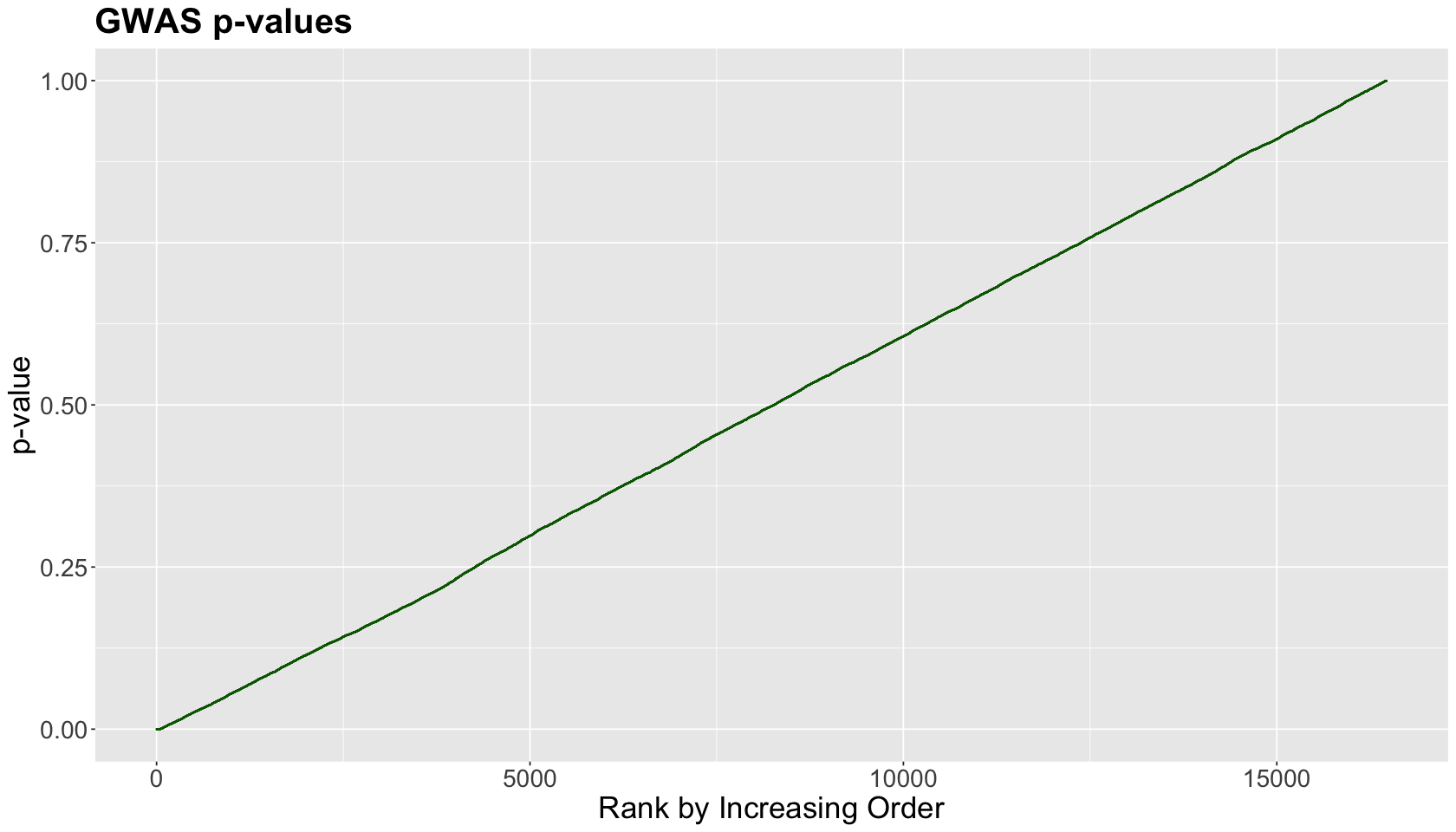
Given the plot above, we might wonder: from this set of \(p\)-values, can we find a cutoff to label significant versus non-significant findings? The FDR will automate finding the “bend in the curve”.
One method to control the FDR is Benjamini-Hochberg (BH). Suppose you have \(m\) hypothesis testings. The method has four steps:
Specify a maximum tolerable FDR, \(\delta\).
Sort the \(m\) p-values from lowest to highest (most significant to least):
Let \(k^*\) be the biggest \(k\) for which \(p_{(k)} < (\delta / m) k\)
Take \(p_{(1)}, \dots, p_{(k^*)}\) as your significant findings.
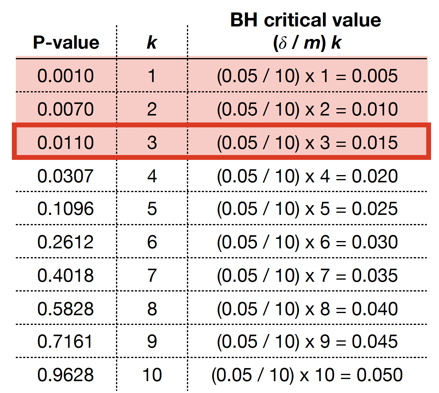
Let us illustrate this procedure with the following raw \(p\)-values:
raw_pvalues <- c(
  0.0010, 0.0070, 0.0110, 0.0307, 0.1096,
  0.2612, 0.4018, 0.5828, 0.7161, 0.9628
)
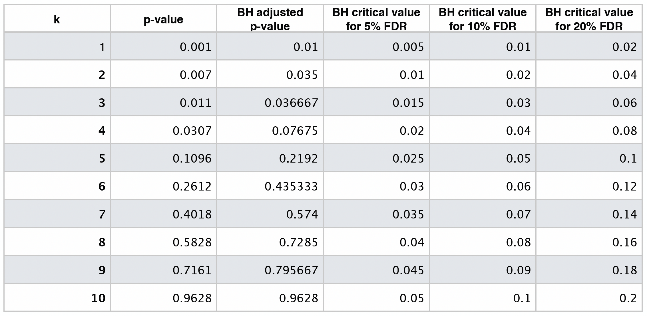
The previous four steps are shown in the table below. Using BH, with \(\delta = 0.05\), we label \(0.0010\), \(0.0070\), and \(0.0110\) as statistically significant via \(k^* = 3\).
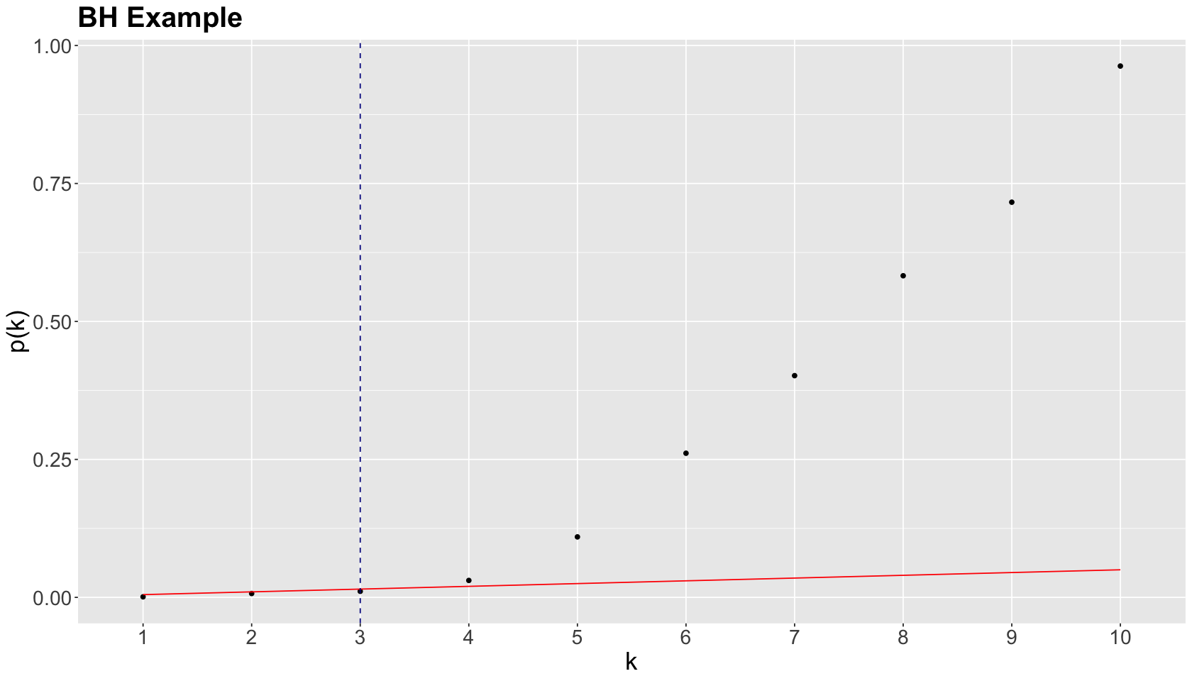
We graphically show the previous BH example below, where each point represents an ordered \(p\)-value. Note the cutoff value is at \(k^* = 3\) (vertical dashed blue line) while the red line corresponds to \((\delta / m) k\) with \(\delta = 0.05\) and \(m = 10\).
pvalues <- data.frame(raw_pvalues, k = seq_along(raw_pvalues)) %>%
  mutate(bh_line = 0.05 / nrow(.) * k)

FDR_plot <- ggplot(pvalues, aes(x = factor(k), y = raw_pvalues)) +
  geom_point() +
  geom_line(aes(x = k, y = bh_line), colour = "red") +
  xlab("k") +
  ylab("p(k)") +
  theme(
    plot.title = element_text(size = 24, face = "bold"),
    axis.text = element_text(size = 17),
    axis.title = element_text(size = 21),
    legend.position = "none"
  ) +
  geom_vline(xintercept = 3, colour = "darkblue", linetype = "dashed") +
  ggtitle("BH Example")
FDR_plot
As in the case of the Bonferroni correction, we can obtain BH adjusted \(p\)-values as
where:
\(i\) is the rank of the raw \(p\)-value.
\(m\) is the number of tests.
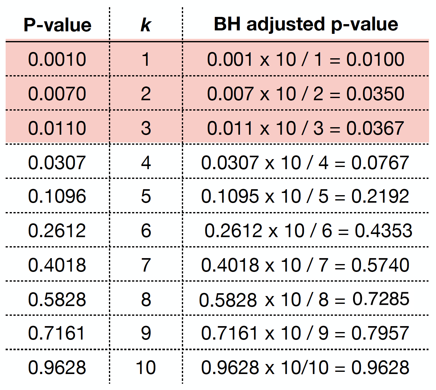
We can obtain the BH adjusted \(p\)-values via p.adjust() as we can see below.
round(p.adjust(raw_pvalues, method = "fdr"), 4)
- 0.01
- 0.035
- 0.0367
- 0.0768
- 0.2192
- 0.4353
- 0.574
- 0.7285
- 0.7957
- 0.9628
By checking these adjusted \(p\)-values, using a maximum tolerable FDR \(\delta = 0.05\), we would label the first three values (from left to right) as statistically significant.
If we want to be even less conservative, i.e. increasing \(\delta\) to 0.10, we would label the first four values as statistically significant.
The table below shows different BH critical values by \(\delta = 0.05, 0.10, 0.20\).
6. Wrapping Up#
So, where do we stand?
If we must make many hypothesis testings without using some \(p\)-value adjustment method, then some spurious findings are expected, just by chance.
There are more than two adjustment methods. However, from these two methods we saw, we should use them as follows:
Bonferroni correction. This method is helpful when there is high confidence all scientific findings correspond to true positives (i.e., we prefer to be very conservative and have false negatives).
FDR. This method is more appropriate if there is a certain proportion of false positives in our scientific findings, and we want to set up a certain level of tolerance (i.e., we prefer to be less conservative and have false positives).
\(H_0\) is true |
\(H_0\) is not true |
|
|---|---|---|
Fail to reject \(H_0\) |
Correct (TRUE NEGATIVE) |
Type II Error (FALSE NEGATIVE) |
Reject \(H_0\) |
Type I Error (FALSE POSITIVE) |
Correct (TRUE POSITIVE) |