Lecture 4 - More Blocking and Power

Lecture 4 - More Blocking and Power#

Today’s Learning Objectives#

Propose the use of control, blocking, randomization, and replication in the design of an A/B testing.
Contrast the performance of blocking versus non-blocking designs with increasing overall sample sizes.
Relate the statistical notion of power to the real-world utility of an experiment in an A/B testing sample size computation.
Contrast the performance of blocking versus non-blocking designs in terms of block homogeneity.

Loading `R` Packages#

options(repr.matrix.max.rows = 8)
library(tidyverse)
library(broom)
library(cowplot)
library(scales)
library(pwr)
library(reshape2)

Previously…#

In Lecture 3 - Randomization and Blocking, we considered blocking in our experimental design versus non-blocking and their associated modelling frameworks. Blocking can be our friend if we consider it from the first experimental stages (i.e., when planning our experiment!). Note you need to clearly know how your population is stratified (more on this matter in Blocking and Stratification).

Nevertheless, we need to explore other essential matters when trying A/B testing. For instance:

How large should our overall sample size be to have an acceptable power?
Will we be able to capture a given treatment effect of “business importance”?
If we use a blocking design, what characteristics should our blocks have?

1. Blocking Simulation Setup#

Let us retake our simulation from Lecture 3 - Randomization and Blocking to elaborate on the concepts we will see today.

1.1. Main Statisical Inquiry#

You aim to run an A/B testing on a subscription website to experiment with a new layout (i.e., the experimental treatment) to increase the mean duration time (hours) on your website (i.e., the response). You will compare this new layout versus the existing one (i.e., the control treatment). Therefore, you will have an experimental factor of interest with two levels: current versus new layout.

1.2. Experimental Limitations and Secondary Statistical Inquiry#

This time, the company does not have enough budget for a sample size of $n = 200$ customers. They can only afford an A/B testing with $n = 100$ customers. Hence, as an additional inquiry, what are the implications on the A/B testing’s estimates and conclusions under this sample size reduction?

1.3. Function for Synthetic Data#

Recall we will have ten demographic categories (or blocks). Each one of these categories will have a different mean duration time on your website. For the $i$th subscriber in the $j$th block, the response $Y_{i,j}$ will be decomposed and simulated as

\[Y_i = 8 + \alpha_{D_{j}} + \theta I_{\text{trt},i} + \varepsilon_{i, j},\]

where:

$Y_{i,j}$ is the subscriber’s duration time on the website.
8 hours is the average duration time on the website for all the current subscribers.
$\alpha_{D_{j}}$ is the $j$th block effect difference (with respect to previous average duration time) which will take on ten values (depending on which block the subscriber belongs to, i.e., $j = 1, \dots, 10$). The between-block variance will be $\sigma_D^2 = 2.5^ 2$.
$\theta$ is our experimental treatment effect of interest, i.e., by how much the response increases/decreases with the new layout compared to the current one.

We will not go over the data simulation step by step. Instead, we will create a function called AB_blocking() whose arguments will be the following:

num_blocks: Number of blocks to simulate in the population.
n: Overall sample size budgeted for the A/B testing.
sd_wthn_blocks: Population within-block standard deviation.
theta: Population experimental treatment effect of interest.
alpha: Population blocking effects.

The function will return two datasets in a list: data_exp_A and data_exp_B. The datasets will come from two different experimental designs:

data_exp_A (non-blocking design): We obtain our sample of $n$ subscribers, and we randomly assign them to either one of the experimental treatments of interest without taking into account the demographic blocks they belong when designing our experiment.
data_exp_B (blocking-design): We randomize our treatments of interest within each of the num_blocks. There is no need to simulate the demographic category in this case since we exactly need n / num_blocks sampled subscribers per block.

Attention

Labels A and B for our experimental designs ARE NOT related to the name A/B testing.

AB_blocking <- function(num_blocks, n, sd_wthn_blocks, theta, alpha) {
  size_block <- n / num_blocks # Block size

  dmg_dist <- seq(from = 5, to = 1, length = num_blocks) # Population's blocking distribution
  dmg_dist <- dmg_dist / sum(dmg_dist)

  # Design Strategy A
  # We directly sample n subscribers from the population
  # Balanced randomization by experimental treatment of interest (no blocking!)
  treat_exp_A <- sample(c(rep(0, n / 2), rep(1, n / 2)))
  # We need to simulate the demographic category (1 to n_num_blocks) to construct
  # our response y using the discrete probability distribution dmg_dist
  dmg_exp_A <- sample(1:num_blocks, size = n, prob = dmg_dist, replace = T)
  # Building our responses for experiment A according to the simulation's equation
  y_exp_A <- rnorm(n, mean = 8 + alpha[dmg_exp_A] + theta * treat_exp_A, sd = sd_wthn_blocks)
  # Training set
  data_exp_A <- tibble(x = treat_exp_A, dmg = as.factor(dmg_exp_A), y = y_exp_A) %>%
   mutate(x = as.factor(ifelse(x == 1, "New Layout", "Current Layout")))

  # Design Strategy B
  treat_exp_B <- NULL
  dmg_exp_B <- NULL
  for (i in 1:num_blocks) {
    # Each block has own balanced randomization
    treat_exp_B <- c(treat_exp_B, sample(c(
      rep(0, size_block / 2),
      rep(1, size_block / 2)
    )))
    dmg_exp_B <- c(dmg_exp_B, rep(i, size_block))
  }
  # Building our responses for experiment B according to the simulation's equation
  y_exp_B <- rnorm(n, mean = 8 + alpha[dmg_exp_B] + theta * treat_exp_B, sd = sd_wthn_blocks)
  # Training set
  data_exp_B <- tibble(x = treat_exp_B, dmg = as.factor(dmg_exp_B), y = y_exp_B) %>%
   mutate(x = as.factor(ifelse(x == 1, "New Layout", "Current Layout")))

  # Building list
  sim_datasets <- list(data_exp_A = data_exp_A, data_exp_B = data_exp_B)

  return(sim_datasets)
}

1.4. Simulation and Exploratory Data Analysis#

Let us use our function AB_blocking() to simulate our experimental designs with $n = 100$ per strategy. The rest of the settings remain as in lecture3. Beforehand, we need to set up population blocking effects in alpha (to be used in function AB_blocking()).

set.seed(554)
sd_btwn_blocks <- 2.5 # Population between-block standard deviation
block_effects <- rnorm(n = 10, sd = sd_btwn_blocks) # Simulating block effects
round(block_effects, 2)

2.04
-2.16
-0.09
-4.25
-1.09
1.15
1.01
-1.57
-2.52
-4.91

set.seed(1234)

sim_n_100 <- AB_blocking(
  num_blocks = 10, n = 100,
  sd_wthn_blocks = 0.8,
  theta = 0.5, alpha = block_effects
)

Our simulated datasets by design strategy are shown below (note we still record the dmg category, but we are not blocking our experimental design in sim_n_100$data_exp_A):

sim_n_100$data_exp_A

A tibble: 100 × 3
x	dmg	y
<fct>	<fct>	<dbl>
Current Layout	7	8.5393201
New Layout	2	6.4643359
Current Layout	10	0.9152359
Current Layout	5	6.9498986
⋮	⋮	⋮
New Layout	7	9.617867
New Layout	4	4.517807
New Layout	5	5.945505
Current Layout	2	6.444226

sim_n_100$data_exp_B

A tibble: 100 × 3
x	dmg	y
<fct>	<fct>	<dbl>
New Layout	1	10.792504
Current Layout	1	9.573213
New Layout	1	9.774556
Current Layout	1	9.893636
⋮	⋮	⋮
New Layout	10	4.221277
New Layout	10	3.955441
Current Layout	10	3.520828
Current Layout	10	3.101476

Before proceeding with our respective statistical modelling, let us make an exploratory data analysis (EDA).

options(repr.plot.height = 8, repr.plot.width = 14)

boxplots_data_exp_A <- ggplot(sim_n_100$data_exp_A) +
  geom_boxplot(aes(dmg, y, fill = x)) +
  theme(
    plot.title = element_text(size = 24, face = "bold"),
    axis.text = element_text(size = 17),
    axis.title = element_text(size = 21),
    legend.position = "bottom",
    legend.title = element_text(size = 21, face = "bold", margin = margin(r = 1, unit = "cm")), 
    legend.text = element_text(size = 17, margin = margin(r = 1, unit = "cm"))
  ) +
  ggtitle("Duration Times with Strategy A") +
  xlab("Demographic Category") +
  ylab("Subscriber's Duration Time (hours)") +
  scale_fill_brewer(palette = "Paired", name = "Treatment")

boxplots_data_exp_B <- ggplot(sim_n_100$data_exp_B) +
  geom_boxplot(aes(dmg, y, fill = x)) +
  theme(
    plot.title = element_text(size = 24, face = "bold"),
    axis.text = element_text(size = 17),
    axis.title = element_text(size = 21),
    legend.position = "bottom",
    legend.title = element_text(size = 21, face = "bold", margin = margin(r = 1, unit = "cm")), 
    legend.text = element_text(size = 17, margin = margin(r = 1, unit = "cm"))
  ) +
  ggtitle("Duration Times with Strategy B") +
  xlab("Demographic Category") +
  ylab("Subscriber's Duration Time (hours)") +
  scale_fill_brewer(palette = "Paired", name = "Treatment")

plot_grid(boxplots_data_exp_A, boxplots_data_exp_B)

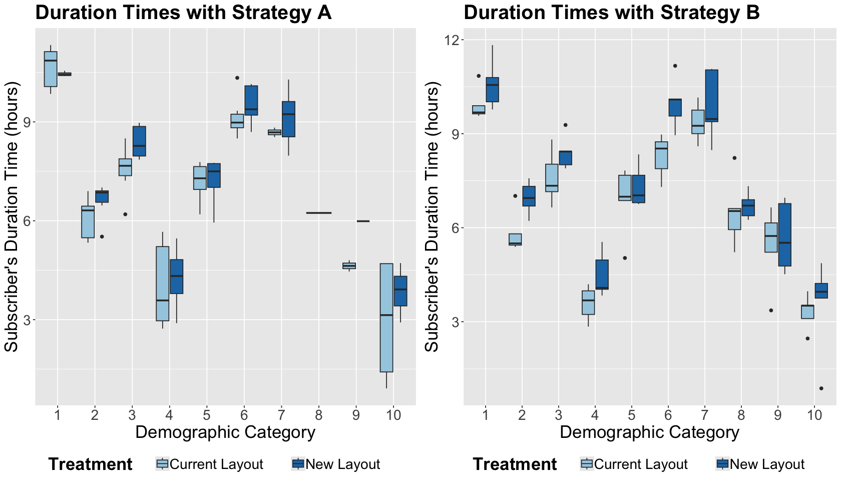
../_images/383540cc7439dbea9772cd7cf1069f2f7cd5708889d6fb4ccaf08f5e4a3de49a.png

Exercise 12

What can we graphically conclude from the previous side-by-side boxplots?

By looking at the below stacked bar charts by absolute frequencies, we highlight the following:

On the right-hand side, we have a balanced representation by demographic category given our randomization design by blocks AND treatments. Thus, we have the same number of observations within each demographic category.
On the left-hand side, the blocks have different subscriber counts by treatment since our randomization design was only done by treatments.

exp_A_stacked_bars <- ggplot(sim_n_100$data_exp_A, aes(dmg, fill = x)) +
  geom_bar(width = 0.7, linewidth = 0.1) +
  xlab("Demographic Category") +
  ylab("Sampled Subscriber Counts") +
  ggtitle("Counts of Sampled Subscribers with Strategy A")  +
  theme(
    plot.title = element_text(size = 20, face = "bold"),
    axis.text = element_text(size = 17),
    axis.title = element_text(size = 20),
    legend.position = "bottom",
    legend.title = element_text(size = 20, face = "bold", margin = margin(r = 1, unit = "cm")), 
    legend.text = element_text(size = 17, margin = margin(r = 1, unit = "cm"))
  ) +
  scale_fill_brewer(palette = "Paired", name = "Treatment") + ylim(0, 20)

exp_B_stacked_bars <- ggplot(sim_n_100$data_exp_B, aes(dmg, fill = x)) +
  geom_bar(width = 0.7, linewidth = 0.1) +
  xlab("Demographic Category") +
  ylab("Sampled Subscriber Counts") +
  ggtitle("Counts of Sampled Subscribers with Strategy B")  +
  theme(
    plot.title = element_text(size = 20, face = "bold"),
    axis.text = element_text(size = 17),
    axis.title = element_text(size = 20),
    legend.position = "bottom",
    legend.title = element_text(size = 20, face = "bold", margin = margin(r = 1, unit = "cm")), 
    legend.text = element_text(size = 17, margin = margin(r = 1, unit = "cm"))
  ) +
  scale_fill_brewer(palette = "Paired", name = "Treatment") + ylim(0, 20)

plot_grid(exp_A_stacked_bars, exp_B_stacked_bars)

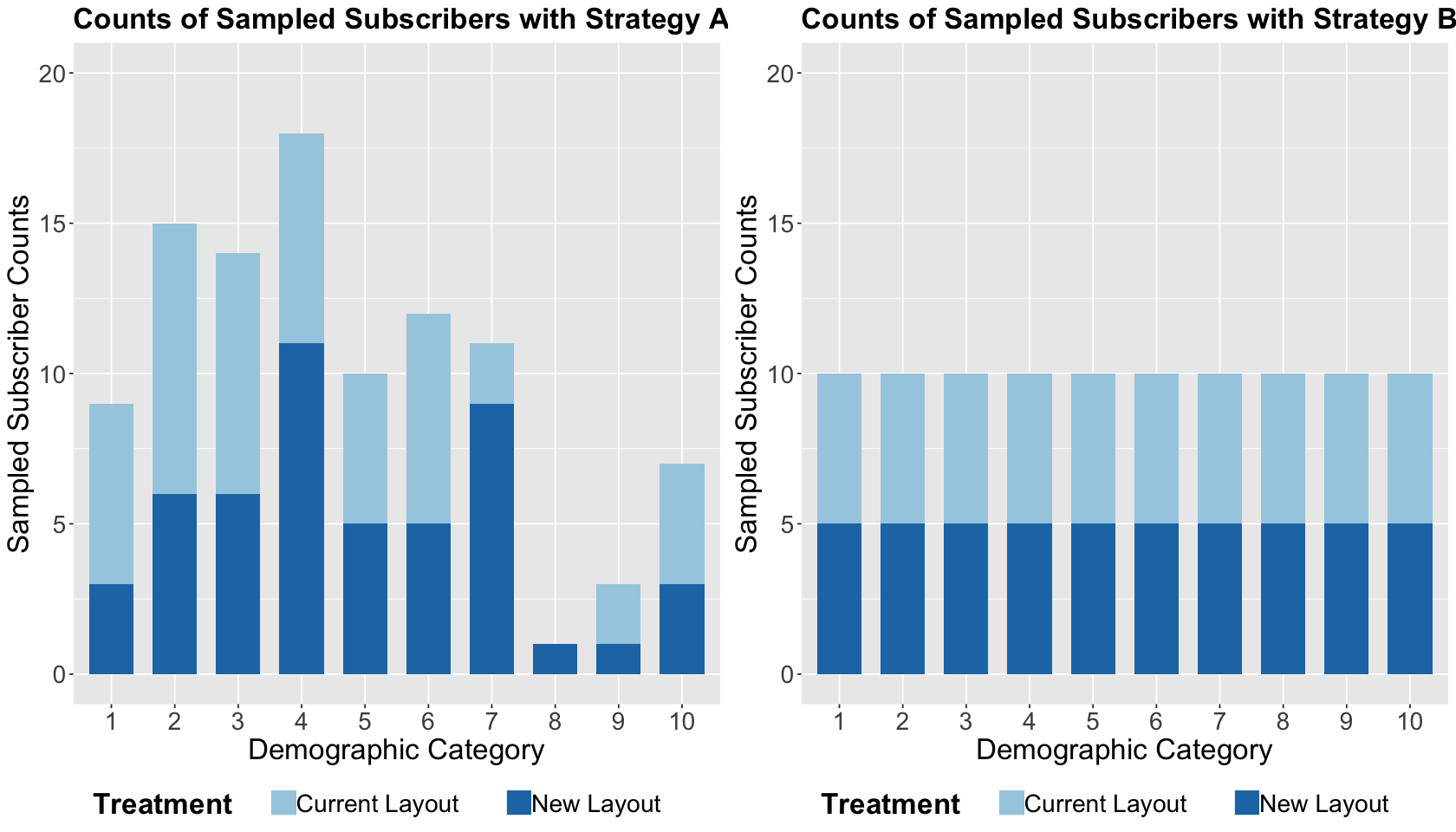
../_images/7cd76fbdc3df567fa6e6d44ab5201be30cbd9fbcf5a50f25e445b3498b229e7d.png

What is the main takeaway from this EDA?

One of the main advantages of blocking design is that we can ensure a sufficient sample representation across the blocking categories, especially with small sample sizes.

1.5. Data Analysis#

As done in Lecture 3 - Randomization and Blocking, we will use the previous simulated datasets to fit the corresponding regression models under three modelling strategies.

Experiment A: Raw Model#

This model will only regress the y on x (current versus new layout), Again, the only significant estimate is the one for the baseline ((Intercept)). The model is not capturing the corresponding effect by demographic category.

exp_A_raw_model_n100 <- lm(y ~ x, data = sim_n_100$data_exp_A) 
tidy(exp_A_raw_model_n100, conf.int = TRUE) %>% mutate_if(is.numeric, round, 2)

A tibble: 2 × 7
term	estimate	std.error	statistic	p.value	conf.low	conf.high
<chr>	<dbl>	<dbl>	<dbl>	<dbl>	<dbl>	<dbl>
(Intercept)	6.91	0.34	20.59	0.00	6.25	7.58
xNew Layout	0.24	0.47	0.51	0.61	-0.70	1.19

Experiment A: Model with Post-Hoc Adjustment for Demographics#

This model still uses the sample from experiment A, but we also include the sample demographic category dmg as a regressor. Note we have an accurate estimate of $\theta$ which is $0.42$ whose 95% confidence interval (CI) is $[0.09, 0.75]$.

options(repr.matrix.max.rows = 15)

exp_A_adj_n100 <- lm(y ~ x + dmg, data = sim_n_100$data_exp_A)
tidy(exp_A_adj_n100, conf.int = TRUE) %>% mutate_if(is.numeric, round, 2)

A tibble: 11 × 7
term	estimate	std.error	statistic	p.value	conf.low	conf.high
<chr>	<dbl>	<dbl>	<dbl>	<dbl>	<dbl>	<dbl>
(Intercept)	10.45	0.27	38.48	0.00	9.91	10.99
xNew Layout	0.42	0.17	2.52	0.01	0.09	0.75
dmg2	-4.34	0.34	-12.91	0.00	-5.01	-3.67
dmg3	-2.70	0.34	-7.93	0.00	-3.38	-2.03
dmg4	-6.52	0.33	-19.84	0.00	-7.18	-5.87
dmg5	-3.48	0.37	-9.47	0.00	-4.21	-2.75
dmg6	-1.34	0.35	-3.80	0.00	-2.04	-0.64
dmg7	-1.72	0.37	-4.69	0.00	-2.45	-0.99
dmg8	-4.63	0.85	-5.46	0.00	-6.32	-2.95
dmg9	-5.51	0.53	-10.36	0.00	-6.56	-4.45
dmg10	-7.28	0.40	-18.11	0.00	-8.08	-6.48

Experiment B: Model with Blocking#

This model uses our data coming from the blocking design. It includes x and dmg as regressors. We have an accurate estimate of $\theta$ of $0.69$ whose 95% CI is $[0.35, 1.03]$.

exp_B_n100 <- lm(y ~ x + dmg, data = sim_n_100$data_exp_B) 
tidy(exp_B_n100, conf.int = TRUE) %>% mutate_if(is.numeric, round, 2)

A tibble: 11 × 7
term	estimate	std.error	statistic	p.value	conf.low	conf.high
<chr>	<dbl>	<dbl>	<dbl>	<dbl>	<dbl>	<dbl>
(Intercept)	9.92	0.28	35.03	0.0	9.35	10.48
xNew Layout	0.69	0.17	4.04	0.0	0.35	1.03
dmg2	-3.87	0.38	-10.14	0.0	-4.63	-3.11
dmg3	-2.26	0.38	-5.91	0.0	-3.01	-1.50
dmg4	-6.22	0.38	-16.29	0.0	-6.98	-5.46
dmg5	-3.16	0.38	-8.28	0.0	-3.92	-2.40
dmg6	-1.13	0.38	-2.96	0.0	-1.89	-0.37
dmg7	-0.64	0.38	-1.68	0.1	-1.40	0.12
dmg8	-3.65	0.38	-9.56	0.0	-4.41	-2.89
dmg9	-4.69	0.38	-12.30	0.0	-5.45	-3.94
dmg10	-6.84	0.38	-17.91	0.0	-7.59	-6.08

Exercise 13

Recall the true population effect is $\theta = 0.5$. Thus, let us focus the attention on the tidy() output for xNew Layout (i.e., estimate $\hat{\theta}$) for models exp_A_adj_n100 and exp_B_n100.

Regarding their corresponding 95% CIs for xNew Layout, what can we conclude on an inferential level?

Select the correct option:

A. Only model exp_A_adj_n100 provides a precise estimate for $\theta$.

B. Only model exp_B_n100 provides a precise estimate for $\theta$.

C. Both models provide precise estimates for $\theta$.

D. Neither of the models provides precise estimates for $\theta$.

1.6. Increasing the Sample Size to $n = 1000$#

Now, suppose the company allows you to increase the sample size to $n = 1000$. First, let us check whether this sample size increase will allow the Raw Model (no blocking) to provide at least an accurate estimate for $\theta = 0.5$.

set.seed(554)
sim_n_1000 <- AB_blocking(
  num_blocks = 10, n = 1000,
  sd_wthn_blocks = 0.8,
  theta = 0.5, alpha = block_effects
)

exp_A_raw_model_n1000 <- lm(y ~ x, data = sim_n_1000$data_exp_A) 
tidy(exp_A_raw_model_n1000, conf.int = TRUE) %>% mutate_if(is.numeric, round, 2)

A tibble: 2 × 7
term	estimate	std.error	statistic	p.value	conf.low	conf.high
<chr>	<dbl>	<dbl>	<dbl>	<dbl>	<dbl>	<dbl>
(Intercept)	7.04	0.11	66.71	0	6.83	7.25
xNew Layout	0.59	0.15	3.94	0	0.30	0.88

At least, we are obtaining an accurate estimate for $\theta = 0.5$ this time (but not so precise!).

Let us do it with the Model with Post-Hoc Adjustment for Demographics. We still have an accurate estimate of $\theta$, which is $0.54$ but more precise. Its 95% CI is $[0.44, 0.64]$.

exp_A_adj_n1000 <- lm(y ~ x + dmg, data = sim_n_1000$data_exp_A)
tidy(exp_A_adj_n1000, conf.int = TRUE) %>% mutate_if(is.numeric, round, 2)

A tibble: 11 × 7
term	estimate	std.error	statistic	p.value	conf.low	conf.high
<chr>	<dbl>	<dbl>	<dbl>	<dbl>	<dbl>	<dbl>
(Intercept)	10.06	0.07	150.98	0	9.93	10.19
xNew Layout	0.54	0.05	10.67	0	0.44	0.64
dmg2	-4.32	0.09	-46.24	0	-4.50	-4.13
dmg3	-2.21	0.09	-24.21	0	-2.39	-2.03
dmg4	-6.43	0.09	-69.33	0	-6.61	-6.25
dmg5	-3.11	0.10	-31.13	0	-3.30	-2.91
dmg6	-0.90	0.10	-8.89	0	-1.10	-0.70
dmg7	-1.10	0.11	-9.73	0	-1.33	-0.88
dmg8	-3.65	0.12	-30.66	0	-3.88	-3.42
dmg9	-4.65	0.14	-33.32	0	-4.92	-4.38
dmg10	-6.90	0.13	-52.27	0	-7.16	-6.64

Finally, the Model with Blocking is estimated via the dataset with the blocking design. Again, the estimate of $\theta$ is accurate (i.e, $0.49$) with a more precise 95% CI of $[0.39, 0.58]$

exp_B_n1000 <- lm(y ~ x + dmg, data = sim_n_1000$data_exp_B) 
tidy(exp_B_n1000, conf.int = TRUE) %>% mutate_if(is.numeric, round, 2)

A tibble: 11 × 7
term	estimate	std.error	statistic	p.value	conf.low	conf.high
<chr>	<dbl>	<dbl>	<dbl>	<dbl>	<dbl>	<dbl>
(Intercept)	10.03	0.08	122.62	0	9.87	10.19
xNew Layout	0.49	0.05	9.85	0	0.39	0.58
dmg2	-4.11	0.11	-37.27	0	-4.33	-3.89
dmg3	-2.12	0.11	-19.18	0	-2.33	-1.90
dmg4	-6.15	0.11	-55.73	0	-6.36	-5.93
dmg5	-3.21	0.11	-29.08	0	-3.42	-2.99
dmg6	-0.83	0.11	-7.56	0	-1.05	-0.62
dmg7	-0.90	0.11	-8.12	0	-1.11	-0.68
dmg8	-3.63	0.11	-32.92	0	-3.85	-3.41
dmg9	-4.55	0.11	-41.26	0	-4.77	-4.33
dmg10	-7.01	0.11	-63.53	0	-7.22	-6.79

What is the main takeaway from these simulation replicates when increasing $n$ from $100$ to $1000$?

Increasing the sample size to from $n = 100$ to $1000$ seems to make all modelling strategies accurate when estimating $\theta$ even with the Raw Model A! Recall that this model does not capture the right systematic component of the population, including the stratum effect (i.e., demographic categories). Moreover, the other two strategies (which take into account the demographic categories in their corresponding setups) are more precise.

Exercise 14

Suppose you are in charge of running this A/B testing. Would you be tempted to suggest to your boss that sample sizes should be increased from $n = 100$ to $1000$?

A. Yes.

B. No.

2. Running a Comprehensive Simulation Study with Varying Sample Sizes#

As discussed in Lecture 3 - Randomization and Blocking, running a single simulation replicate is not enough to have a fully robust conclusion on the advantages of increasing the A/B testing sample size.

Hence, using the same three modelling strategies from the previous section, let us run three simulation studies with varying sample sizes $n = 100, 500, 1000$. Each study will have 500 replicates.

Important

We are basically running Monte Carlo simulations!

The average behaviour will be tracked with the following metrics per modelling strategy with $\theta = 0.5$:

BIAS: The average, over the 500 replicates, of $\hat{\theta} - \theta$. The larger the average, the less accuracy.
ROOT-MEAN-SQUARED ERROR (RMSE): The square root of the average (over the 500 replicates) of $(\hat{\theta}-\theta)^{2}$. It has the following characteristics:
- Interpretable as the typical magnitude of estimation error.
- Captures bias and variance involved in the procedure.
COVERAGE: The proportion (among the 500 replicates) of the 95% CIs that contain the true $\theta$ value.
POWER: It is applicable when $\theta \neq 0$. The proportion of the 500 95% CIs that exclude zero.

The code below executes the previous three strategies 500 times (num_replicates).

2.1. Main Statistical Inquiry#

We will run different simulation studies while varying the training sample sizes to fit the corresponding ordinary least-squares (OLS) models by strategy. By running these simulation studies, we want to know how the power improves as we increase the training sample sizes.

2.2. Coding Up and Running the Simulation Studies#

Our previous function AB_blocking() will be helpful to generate the datasets to be used in our three modelling strategies for each simulation replicate. Nonetheless, we need another function to execute each simulation study by sample size. This function will return a data frame with the previously defined metrics.

Thus, the following code sets up the function sim_study() with the same arguments as in AB_blocking() plus the number of replicates to execute in the study num_replicates. The function returns a data frame with the previous metrics per sample size.

sim_study <- function(num_blocks, n, alpha, sd_wthn_blocks, theta, num_replicates) {
  res <- list(NULL) # Setting up matrix with metrics
  res[[1]] <- res[[2]] <- res[[3]] <- matrix(NA, num_replicates, 3)

  for (lp in 1:num_replicates) {
    # Simulating datasets
    sim_datasets <- AB_blocking(
      num_blocks, n,
      sd_wthn_blocks,
      theta, alpha
    )

    # Do the three analyses
    ft_raw <- lm(y ~ x, data = sim_datasets$data_exp_A)
    ft_post_hoc_adj <- lm(y ~ x + dmg, data = sim_datasets$data_exp_A)
    ft_blocking <- lm(y ~ x + dmg, data = sim_datasets$data_exp_B)

    # and the takeaways
    res[[1]][lp, ] <- c(coef(ft_raw)["xNew Layout"], confint(ft_raw)["xNew Layout", ])
    res[[2]][lp, ] <- c(coef(ft_post_hoc_adj)["xNew Layout"], confint(ft_post_hoc_adj)["xNew Layout", ])
    res[[3]][lp, ] <- c(coef(ft_blocking)["xNew Layout"], confint(ft_blocking)["xNew Layout", ])
  }

  # Summaries
  BIAS <- sapply(
    res,
    function(mat) {
      mean(mat[, 1]) - theta
    }
  )
  vrnc <- sapply(res, function(mat) {
    var(mat[, 1])
  })
  CVRG <- sapply(res,
    function(mat, trg) {
      mean((mat[, 2] < trg) & (trg < mat[, 3]))
    },
    trg = theta
  )
  PWR <- sapply(res, function(mat) {
    mean(mat[, 2] > 0)
  })
  RMSE <- sqrt(BIAS^2 + vrnc)

  opt <- cbind(BIAS, RMSE, CVRG, PWR)
  rownames(opt) <- c("Raw Model A (nothing)", "Adjusted Model A (dmg as a covariate)", "Model B (blocking)")

  return(opt)
}

Now, we use our function sim_study() with 500 replicates per study while varying the sample sizes $n = 100, 500, 1000$. Note that the other function arguments are constant across the three studies.

set.seed(1234)

sim_study_n100 <- sim_study(
  num_blocks = 10, n = 100,
  alpha = block_effects, sd_wthn_blocks = 0.8,
  theta = 0.5, num_replicates = 500
)

sim_study_n500 <- sim_study(
  num_blocks = 10, n = 500,
  alpha = block_effects, sd_wthn_blocks = 0.8,
  theta = 0.5, num_replicates = 500
)

sim_study_n1000 <- sim_study(
  num_blocks = 10, n = 1000,
  alpha = block_effects, sd_wthn_blocks = 0.8,
  theta = 0.5, num_replicates = 500
)

2.3. Simulation Results#

The summaries below corresponding the training sizes $n = 100, 500, 1000$.

round(sim_study_n100, 4)

A matrix: 3 × 4 of type dbl
	BIAS	RMSE	CVRG	PWR
Raw Model A (nothing)	-0.0007	0.4741	0.944	0.202
Adjusted Model A (dmg as a covariate)	0.0010	0.1736	0.944	0.820
Model B (blocking)	0.0017	0.1517	0.960	0.892

round(sim_study_n500, 4)

A matrix: 3 × 4 of type dbl
	BIAS	RMSE	CVRG	PWR
Raw Model A (nothing)	-0.0079	0.1984	0.952	0.672
Adjusted Model A (dmg as a covariate)	0.0036	0.0763	0.936	1.000
Model B (blocking)	0.0002	0.0757	0.934	1.000

round(sim_study_n1000, 4)

A matrix: 3 × 4 of type dbl
	BIAS	RMSE	CVRG	PWR
Raw Model A (nothing)	-0.0075	0.1475	0.938	0.936
Adjusted Model A (dmg as a covariate)	-0.0016	0.0483	0.964	1.000
Model B (blocking)	-0.0024	0.0508	0.956	1.000

Exercise 15

What is the main takeaway from these three simulation studies for $n = 100, 500, 1000$ in the context of this population of interest?

2.4. Examining Power with More Granular Sample Sizes#

Our previous simulation studies already concluded that we could achieve an acceptable power level with no more than $n = 500$.

Main Statistical Inquiry

We might be interested in decreasing the sample size $n$ even more in an A/B testing without sacrificing power. Recall the costs associated with a statistical experiment (i.e., A/B testing)!

Let us run another eight simulation studies with $n = 20, 40, 60, 120, 240, 480, 600, 840, 1200$ and examine power. We will still use the function AB_blocking() with the same arguments except for n which will vary in each one of the three modelling strategies: Raw Model A (nothing), Adjusted Model A (dmg as a covariate), Model B (blocking).

There will be 500 replicates by study. The only overall metric to be recorded by study and modelling strategy will be power (the proportion of the 500 95% CIs that exclude zero by modelling strategy).

Important

A high power indicates that our A/B testing is robust enough to detect and estimate an experimental treatment effect (i.e., $\theta$) different from zero.

n_replicates <- 500
sample_size <- c(20, 40, 60, 120, 240, 480, 600, 840, 1200)
n_lev <- length(sample_size)
n_strategy <- 3
pwr <- matrix(NA, n_lev, n_strategy) # Setting up summary matrix

set.seed(554) # Reproducibility
for (i in 1:length(sample_size)) {

  detect <- matrix(0.0, 1, n_strategy)
  
  for (lp in 1:n_replicates) {

    # Simulating datasets
    sim_datasets <- AB_blocking(
      num_blocks = 10, n = sample_size[i],
      sd_wthn_blocks = 0.8,
      theta = 0.5, alpha = block_effects
    )

    # Do the three analyses
    ft_raw <- lm(y ~ x, data = sim_datasets$data_exp_A)
    ft_post_hoc_adj <- lm(y ~ x + dmg, data = sim_datasets$data_exp_A)
    ft_blocking <- lm(y ~ x + dmg, data = sim_datasets$data_exp_B)

    # and the intermediate power calculations
    detect[1] <- detect[1] + (confint(ft_raw)["xNew Layout", 1] > 0)
    detect[2] <- detect[2] + (confint(ft_post_hoc_adj)["xNew Layout", 1] > 0)
    detect[3] <- detect[3] + (confint(ft_blocking)["xNew Layout", 1] > 0)
  }
  
  pwr[i, ] <- detect / n_replicates # Recording power computation by sample size
}

colnames(pwr) <- c("Raw Model A (nothing)", "Adjusted Model A (dmg as a covariate)", "Model B (blocking)")
rownames(pwr) <- paste0("n = ", sample_size)

From the below table, we can see that Model B (blocking) stands out in power for small sample sizes.

options(repr.matrix.max.rows = 20)

pwr

A matrix: 9 × 3 of type dbl
	Raw Model A (nothing)	Adjusted Model A (dmg as a covariate)	Model B (blocking)
n = 20	0.062	0.176	0.246
n = 40	0.106	0.384	0.478
n = 60	0.112	0.604	0.690
n = 120	0.208	0.876	0.912
n = 240	0.364	0.998	0.998
n = 480	0.668	1.000	1.000
n = 600	0.786	1.000	1.000
n = 840	0.904	1.000	1.000
n = 1200	0.952	1.000	1.000

Moreover, we can plot the previous table to get a clearer message.

pwr <- as_tibble(pwr) %>% 
  add_column(sample_size = c(20, 40, 60, 120, 240, 480, 600, 840, 1200))
pwr <- melt(pwr, id = c("sample_size"))

sim_power_plot <- ggplot(pwr, aes(x = sample_size, y = value, colour = variable)) +
  geom_point(size = 4) +
  geom_line(linewidth = 1) +
  theme(
    plot.title = element_text(size = 24, face = "bold"),
    axis.text = element_text(size = 12),
    axis.title = element_text(size = 21),
    legend.position = "bottom",
    legend.title = element_text(size = 21, face = "bold", margin = margin(r = 1, unit = "cm")), 
    legend.text = element_text(size = 17, margin = margin(r = 1, unit = "cm")),
    legend.key.size = unit(2, "cm")
  ) +
  labs(x = "Overall Sample Size n", y = "Power") +
  coord_cartesian(xlim = c(20, 1200), ylim = c(0, 1)) +
  scale_y_continuous(breaks = seq(0, 1, 0.1)) +
  scale_x_continuous(breaks = sample_size) +
  ggtitle("A/B Testing Power (Blocking versus Non-Blocking)") +
  scale_colour_brewer(palette = "Dark2", name = "Model")

sim_power_plot

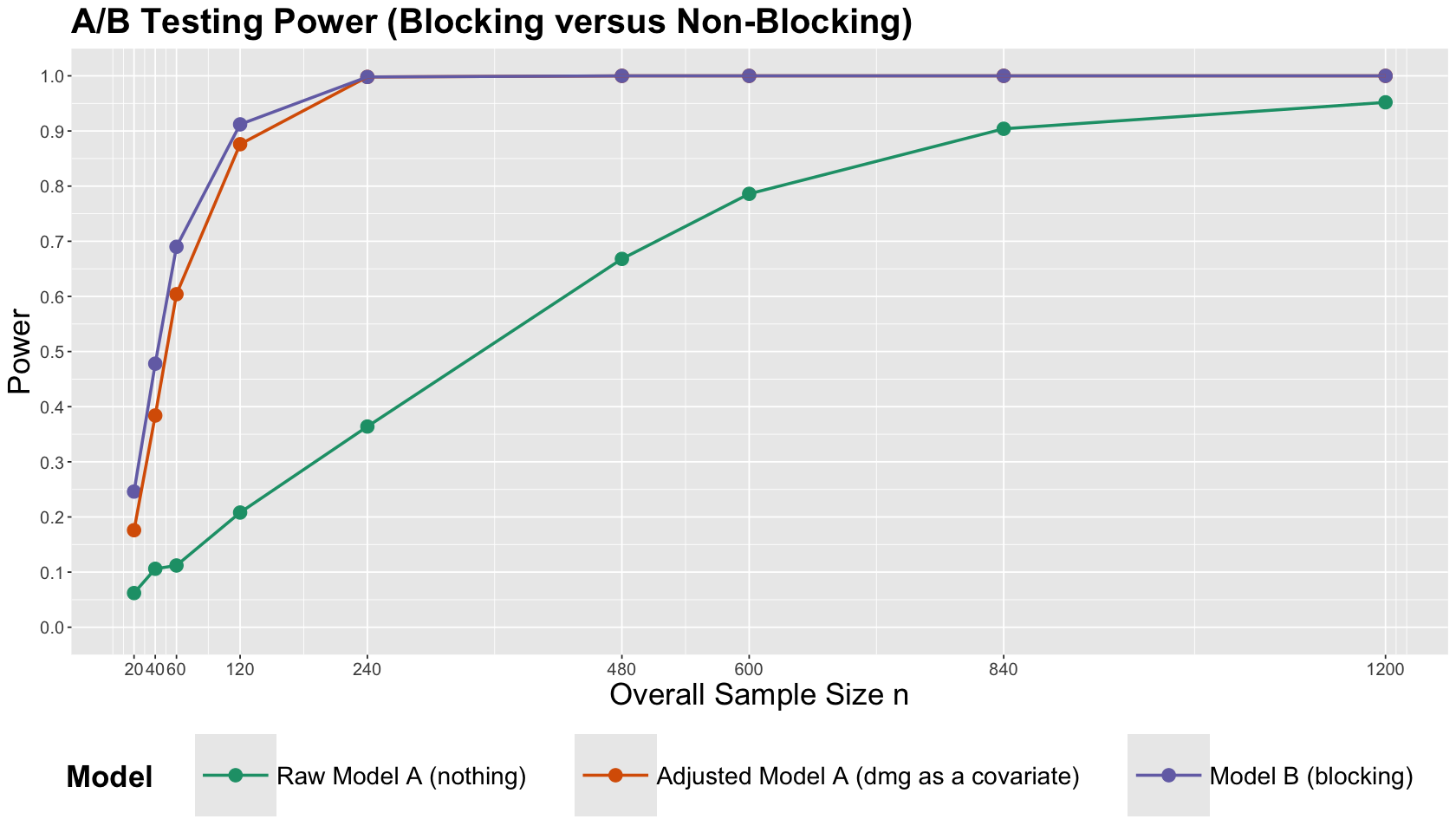
../_images/7c70e00ebf1ed77128618eeeae20458d5bf250f791b18eb8bfc0560e267f9b2b.png

Exercise 16

What is the main takeaway from these simulation studies in the context of this population of interest?

3. Power in Sample Size Computation in `R`#

In this section of the lecture, we will put aside simulations and start exploring R ready-to-be-used formulas to compute sample sizes in A/B testing involving a continuous response $Y$ with a two-level factor $X$.

Recall that sample size computations involve playing around with three concepts:

effect size (how much we want the experimental treatment to differ from the control treatment in terms of the mean response),
significance level $\alpha$, and
the power of the test $1 - \beta$.

3.1. Power and Alpha Trade-Off#

Recall that we set the significance level $\alpha$ to limit the probability of a type I error (falsely rejecting the null hypothesis when in fact is true).

Caution

Imagine you want to be extremely strict with guarding against ever making a Type I error by setting $\alpha = 0$ (never reject the null). However, this would be self-defeating if possible (we already discussed this scenario will never happen), and we would never detect actual departures from the null hypothesis $H_0$ (e.g., we will always fail to reject $H_0$ in this example even though $\theta \neq 0$!).

Recall there is a trade-off between $\alpha$ and the power of the test $1 - \beta$. Now, let us recall the probability $\beta$ is the type II error:

\[\text{Power} = 1 - \beta = 1 - P\{\textrm{do not reject null} \mid \ \textrm{alternative is true}\}.\]

3.2. A Practical Example#

We want to do an A/B testing to see if a tweak (version B) of our existing site (version A) promotes site visitors to stay longer.

Attention

The boss will not sign off on this without some certainty around how many visitors will be randomized to either version A or B.

Suppose we know that CURRENTLY, around 95% of the visitors stay between 30 seconds and 2 minutes. Moreover, we would permanently switch to the tweaked site if we were convinced it improved visit length by 3% (or more!).

Main Statistical Inquiry

Given the problem’s setup, how large should we set up our sample size so we can detect this difference (if there is any!)?

Before using any suitable R function to compute sample sizes, we need to make a distributional assumption on the current visitor’s time. Suppose that for version A, the duration time for the $i$th visitor is

\[Y_i \sim \mathcal{N}(\mu_A, \sigma^2).\]

How do we get $\mu_A$? Recall we know the following:

Suppose we know that CURRENTLY, around 95% of the visitors stay between 30 seconds and 2 minutes.

Assuming this distribution is symmetric (as in the Normal case!), then:

\[\mu_A = 0.5 + \frac{2 - 0.5}{2} = 1.25.\]

We also need to compute $\sigma^2$ if we want to use an R ready-to-be-used formula. Given that we assume normality on $Y_i$, we can use the standardization formula in a Normal random variable:

\[ P(0.5 \leq Y_i \leq 2) = 0.95 \]

\[ P \Bigg( \frac{0.5 - \mu_A}{\sigma} \leq \frac{Y_i - \mu_A}{\sigma} \leq \frac{2 - \mu_A}{\sigma} \Bigg) = 0.95. \]

Note that

\[Z_i = \frac{Y_i - \mu_A}{\sigma} \sim \mathcal{N}(0, 1).\]

We already know that the quantiles that ensure a symmetric 95% coverage in a Standard Normal random variable are

\[ P(-1.96 \leq Z_i \leq 1.96) = 0.95. \]

Therefore, we can obtain $\sigma$ as follows:

\[1.96 = \frac{2 - \mu_A}{\sigma}\]

\[1.96 = \frac{2 - 1.25}{\sigma}\]

\[\sigma = \frac{2 - 1.25}{1.96} = 0.383\]

or equivalently with $-1.96$ and $0.5$

\[\sigma = \frac{0.5 - 1.25}{-1.96} = 0.383.\]

How to we get the desired difference $\delta$ in visit length between the two treatments? Again, let us revisit the inquiry:

Moreover, we would permanently switch to the tweaked site if we were convinced it improved visit length by 3% (or more!).

\[\delta = (\mu_A \times 1.03) - \mu_A = (1.25 \times 1.03) - 1.25 = 0.0375.\]

Attention

The term $\delta$ in this Power Analysis context IS NOT related to the term $\delta$ of the False Discovery Rate (FDR) from Lecture 1 - Multiple Comparisons.

Important

We also need a significance level $\alpha$, which we will set up with the standard value $\alpha = 0.05$. Now, what power do we need? Recall that this is the probability of rejecting the null when the difference is at least $\delta = 0.0375$. A fairly common power choice is

\[1 - \beta = 0.8.\]

Before using the R formula, let us review our sample size computation setup:

We have set a significance level of $\alpha = 0.05$.
We have estimated the standard deviation as $\sigma = 0.383$.
We want detect an effect size of $\delta \geq 0.0375$ at least 80% of the time (power).

The library pwr has the function pwr.t.test(). It needs the following arguments:

d: Desired effect size ($\delta$ divided by $\sigma$).
sig.level: Chosen $\alpha$.
power: Chosen power $1 - \beta$.
type: Type of test (in the A/B testing context we have a two.sample test).
alternative: Our hypothesis test is one-sided, thus greater.

pwr.t.test(
  d = 0.0375 / 0.383,
  sig.level = 0.05,
  power = 0.8,
  type = "two.sample",
  alternative = "greater"
)

     Two-sample t test power calculation 

              n = 1290.509
              d = 0.09791123
      sig.level = 0.05
          power = 0.8
    alternative = greater

NOTE: n is number in *each* group

That is a large sample size by treatment! Hence, you will tell your boss the following:

If we run our experiment with $1291 \times 2 = 2582$ participants in total, then we have a 80% chance (or more) of being convinced of a difference between the two treatment groups, provided that the population difference truly is $0.0375$ (or greater).

It is likely your boss will be surprised with that sample size. Thus, they might be asking for another experimental setup options. And of course, you can provide options:

$\alpha:$ more strict ($0.01$), conventional value ($0.05$), and liberal ($0.1$). The larger the $\alpha$, the more prone we will be to commit type I error.
$1 - \beta$ (power): $0.5$ to $0.9$ by $0.05$. The larger the power, the less prone we will be to commit type II error.
$\delta$: Possibly an increase $\delta = 0.0375$ is too small. We could also try $\delta = 0.05, 0.1$.

# Let us obtain all the possible setting combinations
alpha <- c(0.01, 0.05, 0.1)
power <- seq(from = 0.5, to = 0.9, by = 0.05)
delta <- c(0.0375, 0.05, 0.1)
experimental_grid <- expand.grid(alpha, power, delta)
colnames(experimental_grid) <- c("alpha", "power", "delta")
# Adding a column for the overall sample size n
experimental_grid$overall_n <- NA
experimental_grid

A data.frame: 81 × 4
alpha	power	delta	overall_n
<dbl>	<dbl>	<dbl>	<lgl>
0.01	0.50	0.0375	NA
0.05	0.50	0.0375	NA
0.10	0.50	0.0375	NA
0.01	0.55	0.0375	NA
0.05	0.55	0.0375	NA
0.10	0.55	0.0375	NA
0.01	0.60	0.0375	NA
0.05	0.60	0.0375	NA
0.10	0.60	0.0375	NA
0.01	0.65	0.0375	NA
⋮	⋮	⋮	⋮
0.10	0.75	0.1	NA
0.01	0.80	0.1	NA
0.05	0.80	0.1	NA
0.10	0.80	0.1	NA
0.01	0.85	0.1	NA
0.05	0.85	0.1	NA
0.10	0.85	0.1	NA
0.01	0.90	0.1	NA
0.05	0.90	0.1	NA
0.10	0.90	0.1	NA

# Trying all settings from our previous grid

for (i in 1:nrow(experimental_grid)) {
  # Using sample size function
  sample_size <- tidy(pwr.t.test(
    d = experimental_grid[i, "delta"] / 0.383,
    sig.level = experimental_grid[i, "alpha"],
    power = experimental_grid[i, "power"],
    type = "two.sample",
    alternative = "greater"
  ))

  # Recording overal sample size
  experimental_grid[i, "overall_n"] <- 2 * ceiling(sample_size$n)
}

Note the whole table of 81 sample sizes might be hard to work with.

experimental_grid

A data.frame: 81 × 4
alpha	power	delta	overall_n
<dbl>	<dbl>	<dbl>	<dbl>
0.01	0.50	0.0375	2262
0.05	0.50	0.0375	1132
0.10	0.50	0.0375	688
0.01	0.55	0.0375	2512
0.05	0.55	0.0375	1310
0.10	0.55	0.0375	828
0.01	0.60	0.0375	2780
0.05	0.60	0.0375	1506
0.10	0.60	0.0375	984
0.01	0.65	0.0375	3072
⋮	⋮	⋮	⋮
0.10	0.75	0.1	226
0.01	0.80	0.1	592
0.05	0.80	0.1	366
0.10	0.80	0.1	266
0.01	0.85	0.1	668
0.05	0.85	0.1	424
0.10	0.85	0.1	318
0.01	0.90	0.1	768
0.05	0.90	0.1	504
0.10	0.90	0.1	388

Therefore, let us make a clever plotting arrangement: the so-called Power Analysis plots.

sample_size_power_plot <- ggplot(experimental_grid, aes(x = power, y = overall_n, colour = as.factor(delta))) +
  geom_point(size = 4) +
  geom_line(linewidth = 1) +
  theme(
    plot.title = element_text(size = 24, face = "bold"),
    axis.text = element_text(size = 13.5),
    axis.title = element_text(size = 21),
    strip.text = element_text(size = 21),
    legend.position = "bottom",
    legend.title = element_text(size = 21, face = "bold", margin = margin(r = 1, unit = "cm")), 
    legend.text = element_text(size = 17, margin = margin(r = 1, unit = "cm")),
    legend.key.size = unit(2, "cm")
  ) +
  labs(x = "Power", y = "Overall Sample Size n") +
  coord_cartesian(xlim = c(0.5, 0.9), ylim = c(0, 5500)) +
  scale_y_continuous(breaks = seq(0, 5500, 500)) +
  scale_x_continuous(breaks = power) +
  labs(colour = "Minute Response Increase\nwith Experimental Treatment B\n(% increase in brackets)") +
  ggtitle(expression("A/B Testing Power Analysis with"~alpha~"= 0.01, 0.05, 0.1")) +
  facet_wrap(~ as.factor(alpha)) +
  scale_colour_brewer(palette = "Dark2", labels = c("+0.0375 min (+3%)", "+0.05 min (+4%)", "+0.1 min (+8%)"))

sample_size_power_plot

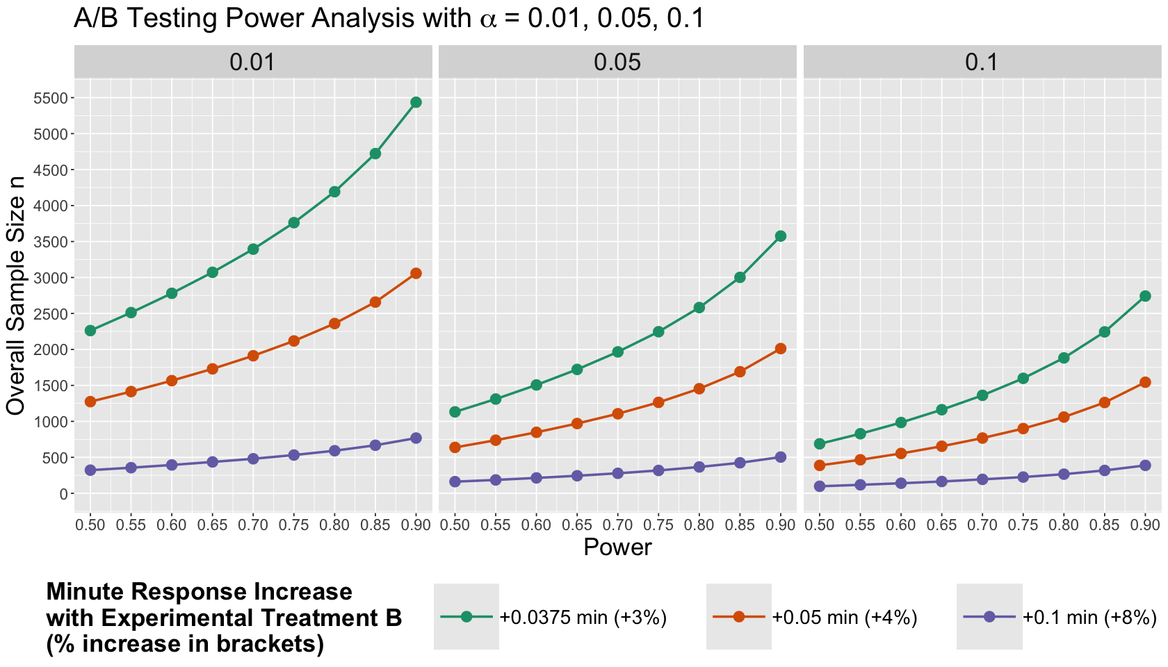
../_images/7c17053ce95d1a7bc4ff0f427d1e4cec780f8f7af1cfd119a65365b946db0cb8.png

What are the main takeaways from this Power Analysis?

If we are incredibly optimistic about the potential success of our experimental treatment (i.e., large $\delta = 0.1$), then the required overall sample size $n$ will be small.
A more strict $\alpha$ dramatically increases the required overall $n$.
The more power, the more sample size we need!

4. Block Homogeneity and Power#

This is our final simulation study using today’s initial case. We will dig more into the following ideas we mentioned in Lecture 3 - Randomization and Blocking:

An important matter to consider regarding blocking is that this strategy will work as long as the blocks are really homogeneous. This implicates stratifying the experimental units into blocks so that:

As much variation in $Y$ as possible is across the blocks.

As little variation in $Y$ as possible is within the blocks.

Hence, you might wonder: what do these statements imply in our experimental design an analysis IN TERMS OF POWER?

To illustrate the previous ideas, let us tweak our modelling setup using our function sim_study() to get the corresponding summary metrics.

4.1. Scenario 1: Well-Defined Blocks with Low Internal Variability#

Suppose that the strata in your population are really well-defined so the corresponding between-block standard deviation is high enough (e.g., 3) in terms of our response of interest (subscriber’s duration time on the website). On the other hand, the experimental units within each block are really similar (i.e., homogeneous!) in terms of the response of interest. Therefore, the within-block standard deviation is low enough (e.g., 0.5)

Let us run the simulation study with a training size n of 100, 10 blocks, a population $\theta = 0.5$, and 500 replicates.

set.seed(554) # Reproducibility
sd_btwn_blocks_1 <- 3 # Population between-block standard deviation
block_effects_1 <- rnorm(n = 10, sd = sd_btwn_blocks_1) # Simulating block effects
round(block_effects_1, 2)

2.44
-2.6
-0.1
-5.1
-1.31
1.38
1.21
-1.89
-3.02
-5.89

sim_study_homogeneous_blocks <- sim_study(
  num_blocks = 10, n = 100,
  alpha = block_effects_1, sd_wthn_blocks = 0.5,
  theta = 0.5, num_replicates = 500
)

4.2. Scenario 2: Poor-Defined Blocks with High Internal Variability#

Now, let us switch the variabilities. Suppose the strata are not well-defined. Thus, the between-block standard deviation is low (e.g., 0.5) in our response of interest. Furthermore, there is a lot of variability within the experimental units in the block (i.e., the block leans more to being heterogeneous). This matter will be translated into a high within-block standard deviation (e.g. 3).

set.seed(554) # Reproducibility
sd_btwn_blocks_2 <- 0.5 # Population between-block standard deviation
block_effects_2 <- rnorm(n = 10, sd = sd_btwn_blocks_2) # Simulating block effects
round(block_effects_2, 2)

0.41
-0.43
-0.02
-0.85
-0.22
0.23
0.2
-0.31
-0.5
-0.98

sim_study_non_homogeneous_blocks <- sim_study(
  num_blocks = 10, n = 100,
  alpha = block_effects_2, sd_wthn_blocks = 3,
  theta = 0.5, num_replicates = 500
)

4.3. Comparing Both Scenarios#

Now, let us check the numerical summaries:

round(sim_study_homogeneous_blocks, 3)

A matrix: 3 × 4 of type dbl
	BIAS	RMSE	CVRG	PWR
Raw Model A (nothing)	0.016	0.541	0.932	0.166
Adjusted Model A (dmg as a covariate)	-0.003	0.104	0.956	0.994
Model B (blocking)	-0.004	0.098	0.948	0.998

round(sim_study_non_homogeneous_blocks, 3)

A matrix: 3 × 4 of type dbl
	BIAS	RMSE	CVRG	PWR
Raw Model A (nothing)	0.002	0.590	0.960	0.118
Adjusted Model A (dmg as a covariate)	-0.015	0.622	0.956	0.122
Model B (blocking)	-0.026	0.589	0.948	0.098

What is the main takeaway from these simulation studies in the context of this population and power?

Blocking can be less beneficial if the within-block variation is (a lot!) higher than the between-block variation. Hence, we have to be extremely cautious when designing our A/B testing if we decide to go ahead with blocking. The blocking setup needs to be carefully planned before running the experiment.

5. Wrapping Up#

Blocking can give us a boost in power, especially for small sample sizes.
So can include relevant covariates in our regression model, even with a randomized experiment!
Power quantifies our ability to detect effects that really are there.
For a desired power, we can calculate the required sample size.
An important block characteristic is its clear definition in terms of the response of interest, i.e., we have to make sure our blocks are appropriately defined.

Lecture 4 - More Blocking and Power

Contents

Lecture 4 - More Blocking and Power#

Today’s Learning Objectives#

Loading `R` Packages#

Previously…#

1. Blocking Simulation Setup#

1.1. Main Statisical Inquiry#

1.2. Experimental Limitations and Secondary Statistical Inquiry#

1.3. Function for Synthetic Data#

1.4. Simulation and Exploratory Data Analysis#

1.5. Data Analysis#

Experiment A: Raw Model#

Experiment A: Model with Post-Hoc Adjustment for Demographics#

Experiment B: Model with Blocking#

1.6. Increasing the Sample Size to \(n = 1000\)#

2. Running a Comprehensive Simulation Study with Varying Sample Sizes#

2.1. Main Statistical Inquiry#

2.2. Coding Up and Running the Simulation Studies#

2.3. Simulation Results#

2.4. Examining Power with More Granular Sample Sizes#

3. Power in Sample Size Computation in `R`#

3.1. Power and Alpha Trade-Off#

3.2. A Practical Example#

4. Block Homogeneity and Power#

4.1. Scenario 1: Well-Defined Blocks with Low Internal Variability#

4.2. Scenario 2: Poor-Defined Blocks with High Internal Variability#

4.3. Comparing Both Scenarios#

5. Wrapping Up#

Lecture 4 - More Blocking and Power

Contents

Lecture 4 - More Blocking and Power#

Today’s Learning Objectives#

Loading R Packages#

Previously…#

1. Blocking Simulation Setup#

1.1. Main Statisical Inquiry#

1.2. Experimental Limitations and Secondary Statistical Inquiry#

1.3. Function for Synthetic Data#

1.4. Simulation and Exploratory Data Analysis#

1.5. Data Analysis#

Experiment A: Raw Model#

Experiment A: Model with Post-Hoc Adjustment for Demographics#

Experiment B: Model with Blocking#

1.6. Increasing the Sample Size to \(n = 1000\)#

2. Running a Comprehensive Simulation Study with Varying Sample Sizes#

2.1. Main Statistical Inquiry#

2.2. Coding Up and Running the Simulation Studies#

2.3. Simulation Results#

2.4. Examining Power with More Granular Sample Sizes#

3. Power in Sample Size Computation in R#

3.1. Power and Alpha Trade-Off#

3.2. A Practical Example#

4. Block Homogeneity and Power#

4.1. Scenario 1: Well-Defined Blocks with Low Internal Variability#

4.2. Scenario 2: Poor-Defined Blocks with High Internal Variability#

4.3. Comparing Both Scenarios#

5. Wrapping Up#

Loading `R` Packages#

3. Power in Sample Size Computation in `R`#