Lecture 7 - Observational Data: Different Sampling Schemes

Lecture 7 - Observational Data: Different Sampling Schemes#

Today’s Learning Objectives#

Introduce the use of different sampling schemes in observational studies.
Illustrate the concept of the proxy ground truth to assess different sampling schemes.
Apply complete simulation studies to a given sampling scheme via the proxy ground truth.
Explore the efficiency of the Case-Control sampling scheme via a modified power analysis.

Loading `R` Packages#

options(repr.matrix.max.rows = 8, repr.matrix.max.cols = 10)
library(foreign)
library(tidyverse)
library(broom)
library(reshape2)

Previously…#

We introduced observational studies to assess causality between a variable \(X\) and a response \(Y\). Moreover, we highlighted that observational studies are used when randomized experimentation is infeasible. Hence, an observational study would try to make the best for data involving \(X\), \(Y\), and \(p\) confounders \(C_j\) (\(i = 1, \dots, p\)).

In Lecture 6 - Observational Data: Stratifying and Modelling, we reviewed a case study that followed two strategies:

Stratum-specific causal inference with multiple confounders. We stratified our data according to the confounders \(C_j\) to see how \(X\) and \(Y\) are related (primarily in a causation framework) within homogeneous strata. However, we encountered different estimation problems while following this approach since not all strata had sufficient absolute frequencies by cell in their respective contingency tables.
Overall Model-Based Causal Inference. We pursued an overall model-based causal inference which is basically a regression of \(Y\) using \(X\) and \(C_{1}, \ldots, C_{p}\) as regressors. This approach proved to be more effective since we controlled for the possible confounders in our model. Therefore, we assumed that no matter what confounders a population of interest had as long as we control them in our regression’s systematic component, all subjects would have the same effect of \(X\) over \(Y\).

Recall the overall model-based causal inference required three fundamental assumptions:

No interactions between strata, which implies a simple/smooth structure in how \(Y\) varies across strata (i.e., not including all possible interactions between the \(p\) confounders at any degree).
No interactions involving \(X\) and any confounder \(C_j\), which implies that the strength of the \((X, Y)\) association within strata does not vary across strata.
Have we captured all confounders in our selection of \(C_{1}, \ldots, C_{p}\)? A challenging assumption to fulfill!

As we can see, we have already seen causal analysis in observational studies. Therefore, it is time to check causal design in observational studies.

1. Sampling Schemes in Observational Studies#

We will build on what we did in Lecture 6 - Observational Data: Stratifying and Modelling by looking at different sampling schemes for observational data.

Attention

This is an important lecture since this is the first time we dig deeper into the field of statistical sampling.

As in randomized experiments (i.e., non-blocking versus blocking), there are different ways we can gather our data in observational studies. Mainly, we must explore how to select our sample before executing the study. Moreover, our subsequent statistical analysis needs to account for how we sample our data.

1.1. Sampling Assessment Via the Ground Truth#

Besides evaluating our statistical modelling (as we did via the three assumptions we explored in Lecture 6 - Observational Data: Stratifying and Modelling, we also need to assess any given sampling scheme before executing it.

Nonetheless, how are we supposed to evaluate these schemes? We need to introduce a new concept to explain this matter. It is called the ground truth.

Important

In Statistics and Machine Learning, the ground truth implicates checking the results of any given approach (e.g., a sampling scheme and its corresponding statistical model in the form of regression) in terms of its estimation accuracy against the real-world.

Nevertheless, assessing our methods in statistical inference is challenging because we do not have a concrete ground truth! Under the frequentist paradigm, since we DO NOT have access to the population data, we only rely on a sample (hopefully representative!) which we use to estimate fixed population parameters. Hence, the ground truth will not be available!

Not having access to the ground truth will be especially problematic if we want to infer something more complex than variable association, i.e., we would like to infer causality between \(X\) and \(Y\). However, we are now familiar with a powerful tool to build a proxy of the ground truth: simulation.

1.2. Simulation: A Proxy of the Ground Truth#

We have been using basic Monte Carlo simulation throughout this block. However, we will use a more sophisticated simulation technique throughout this lecture. The core ideas of this technique are the following:

Use a relevant sample dataset. This step assumes a previous sample dataset as representative enough of our population of interest. Ideally, we want our sampling methods to work on data with the typical characteristics of this population.
Fit a model. We will use the relevant sample dataset to fit a model of the response \(Y\) versus the variable \(X\) and a determined set of confounders \(C_j\) (as strata).
Simulate a proxy ground truth. This step will use the model from step 2 to simulate new outcomes \(Y\). Basically, we would keep the same regressors’ ranges since we are using their corresponding fitted model to simulate new observations. These are the typical ranges we would encounter in real population data.

Attention

The previous steps will use the three assumptions from Lecture 6 - Observational Data: Stratifying and Modelling in two ways:

The first way will come in step 2 since we will have to use the model we concluded was the “best one” (\(Y\), \(X\), and a given set of confounders as strata).
The second way will use these assumptions when generating new data in step 3 via the model from step 2.

Exercise 23

Answer TRUE or FALSE:

We could visualize the previous process of building a proxy ground truth as a modified bootstrapping taken to a higher level.

A. TRUE

B. FALSE

2. The Western Collaborative Group Study Data#

We will retake the Western Collaborative Group Study (WCGS) data to illustrate the previously defined three-step process. The WCGS data is a prospective cohort study that recruited middle-aged men between the ages of 39 and 59 who were employees of ten Californian companies. The data was collected on 3154 subjects between 1960 and 1961.

Caution

Before continuing with our three-step process to build a proxy for the ground truth, we need to clarify that we will use it as representative data from our population of interest.

2.1. Step 1: Use a Relevant Sample Dataset#

We initially load our data. Then, we will eliminate those rows with missing data via na.omit() (missing data will again not be the scope of today’s lecture!). We end up with \(3,101\) subjects.

wcgs <- as_tibble(read.dta("../data/wcgs.dta"))
wcgs <- na.omit(wcgs)
wcgs

A tibble: 3101 × 22
age	arcus	behpat	bmi	chd69	⋯	typchd69	uni	weight	wghtcat	agec
<int>	<int>	<fct>	<dbl>	<fct>	⋯	<int>	<dbl>	<int>	<fct>	<fct>
50	1	A1	31.32101	No	⋯	0	0.4860738	200	170-200	46-50
51	0	A1	25.32858	No	⋯	0	0.1859543	192	170-200	51-55
59	1	A1	28.69388	No	⋯	0	0.7277991	200	170-200	56-60
51	1	A1	22.14871	No	⋯	0	0.6244636	150	140-170	51-55
⋮	⋮	⋮	⋮	⋮	⋱	⋮	⋮	⋮	⋮	⋮
41	0	B4	25.03378	No	⋯	0	0.27816987	195	170-200	41-45
53	0	B4	25.79944	No	⋯	0	0.95139700	185	170-200	51-55
54	0	B4	23.49076	No	⋯	0	0.57082593	150	140-170	51-55
48	0	B4	30.26990	No	⋯	0	0.08677829	205	> 200	46-50

The three assumptions from Lecture 6 - Observational Data: Stratifying and Modelling will come into play in this part. Suppose the following model was the “best one” (note age, bmi, smoke, and chol are used as strata):

glm(chd69 ~ dibpat + age_bins + smoke + bmi_bins + chol_bins, family = "binomial", data = wcgs)

Thus, we select the following variables from wcgs:

dibpat: Dichotomous behaviour pattern, a factor-type variable with two levels (Type A and Type B).
age: Subject’s age in years (a count-type variable).
bmi: Subject’s body mass index (BMI) in \(\text{kg}/\text{m}^2\) (a continuous-type variable).
chol: Subject’s cholesterol levels in \(\text{mg}/100 \text{ ml}\) (a continuous-type variable).
smoke: Whether the subject smokes or not, a factor-type variable with two levels (Yes and No).
chd69: Whether the subject experienced a coronary heart disease (CHD) event, a factor-type variable with two levels (Yes and No).

wcgs <- wcgs %>%
  select(dibpat, age, bmi, chol, smoke, chd69)

Recall the main statistical inquiry of this causal model:

Does a Type A behaviour pattern (dibpat) LEAD to a coronary heart disease (CHD) event (chd69)?

From Brand et al. (1976), the levels of dibpat are defined as follows:

Methods for the assessment of the dichotomous behavior pattern by a structured psychological interview in the WCGS have been described elsewhere. Type A behavior is characterized by enhanced aggressiveness and competitive drive, preoccupation with deadlines, and chronic impatience and sense of time urgency, in contrast with the more relaxed and less hurried Type B behavior pattern.

Therefore \(Y\) will be chd69 and \(X\) will be dibpat, whereas age, bmi, chol and smoke will be confounders in the proxy of the ground truth.

Given the form of the model

glm(chd69 ~ dibpat + age_bins + smoke + bmi_bins + chol_bins, family = "binomial", data = wcgs)

we need to create strata by confounder (except for smoke which is already categorical). These strata will be formed on a quartile basis.

wcgs <- wcgs %>%
  mutate(
    age_bins = cut(age, breaks = c(min(age), quantile(age, (1:3) / 4), max(age)), include.lowest = TRUE),
    bmi_bins = cut(bmi, breaks = c(min(bmi), quantile(bmi, (1:3) / 4), max(bmi)), include.lowest = TRUE),
    chol_bins = cut(chol, breaks = c(min(chol), quantile(chol, (1:3) / 4), max(chol)), include.lowest = TRUE)
  )
wcgs

A tibble: 3101 × 9
dibpat	age	bmi	chol	smoke	chd69	age_bins	bmi_bins	chol_bins
<fct>	<int>	<dbl>	<int>	<fct>	<fct>	<fct>	<fct>	<fct>
Type A	50	31.32101	249	Yes	No	(45,50]	(25.8,38.9]	(223,253]
Type A	51	25.32858	194	Yes	No	(50,59]	(24.4,25.8]	[103,197]
Type A	59	28.69388	258	No	No	(50,59]	(25.8,38.9]	(253,645]
Type A	51	22.14871	173	No	No	(50,59]	[11.2,23]	[103,197]
⋮	⋮	⋮	⋮	⋮	⋮	⋮	⋮	⋮
Type B	41	25.03378	180	No	No	[39,42]	(24.4,25.8]	[103,197]
Type B	53	25.79944	167	No	No	(50,59]	(24.4,25.8]	[103,197]
Type B	54	23.49076	242	Yes	No	(50,59]	(23,24.4]	(223,253]
Type B	48	30.26990	288	No	No	(45,50]	(25.8,38.9]	(253,645]

Once we have all variables ready, we construct a simulated population called sim_pop. This population is based on the fact everyone in dataset wcgs contributes with twenty clones (in terms of \(X\) and \(C_j\)s). We shuffle all rows at the end for subsequent sampling purposes.

Attention

Note we are not using \(Y\) (ch69) to make these clones. We will construct \(Y\) in step 2.

set.seed(554) # Reproducibility

sim_pop <- data.frame(
  dibpat = rep(wcgs$dibpat, each = 20),
  age_bins = rep(wcgs$age_bins, each = 20),
  smoke = rep(wcgs$smoke, each = 20),
  bmi_bins = rep(wcgs$bmi_bins, each = 20),
  chol_bins = rep(wcgs$chol_bins, each = 20)
)
# Shuffling rows!
rows <- sample(nrow(sim_pop))
sim_pop <- sim_pop[rows, ]
sim_pop

A data.frame: 62020 × 5
	dibpat	age_bins	smoke	bmi_bins	chol_bins
	<fct>	<fct>	<fct>	<fct>	<fct>
46844	Type B	[39,42]	No	(24.4,25.8]	(197,223]
36954	Type B	(50,59]	No	(25.8,38.9]	[103,197]
47173	Type B	(42,45]	No	(23,24.4]	[103,197]
44779	Type B	(50,59]	No	(23,24.4]	(197,223]
⋮	⋮	⋮	⋮	⋮	⋮
13998	Type A	(42,45]	No	(25.8,38.9]	[103,197]
43487	Type B	[39,42]	No	[11.2,23]	[103,197]
14393	Type A	(42,45]	Yes	(25.8,38.9]	[103,197]
45693	Type B	(50,59]	Yes	(25.8,38.9]	[103,197]

2.2. Step 2: Fit a Model#

Now, using the sample in wcgs, we will fit a Binary Logistic regression as follows:

wcgs_bin_log_model <- glm(chd69 ~ dibpat + age_bins + smoke + bmi_bins + chol_bins,
  family = "binomial", data = wcgs
)

To mimic the variable structure of the actual dataset wcgs into sim_pop, we will use the estimated regression coefficients from wcgs_bin_log_model to set the “true” relationship between the \(Y\) (chd69) and the \(X\) (dibpat) along with the confounders as strata.

wcgs_coef_pop <- coef(wcgs_bin_log_model)
round(wcgs_coef_pop, 2)

(Intercept): -4.83
dibpatType A: 0.72
age_bins(42,45]: 0.16
age_bins(45,50]: 0.63
age_bins(50,59]: 0.94
smokeYes: 0.64
bmi_bins(23,24.4]: 0.33
bmi_bins(24.4,25.8]: 0.48
bmi_bins(25.8,38.9]: 0.68
chol_bins(197,223]: 0.35
chol_bins(223,253]: 0.88
chol_bins(253,645]: 1.29

2.3. Step 3: Simulate a Proxy Ground Truth#

For the success event in the binary \(Y_i\), we know how to compute predicted probabilities \(\hat{\pi}_i\) given the estimated regression coefficients coming from a trained logistic regression model (such as wcgs_bin_log_model) for the \(i\)th subject:

\[ \hat{\pi}_i = \frac{\exp\big[\mbox{logit}(\pi_i)\big]}{1 + \exp\big[\mbox{logit}(\pi_i)\big]}, \]

where

\[ \mbox{logit}(\hat{\pi}_i) = \hat{\beta}_0 + \hat{\beta}_X X_{i, 1} + \hat{\beta}_1 C_{i, 1} + \ldots + \hat{\beta}_p C_{i, p}. \]

Note that \(\hat{\beta}_X\) corresponds to the estimated regression coefficient for \(X\), whereas \(\hat{\beta}_1, \dots, \hat{\beta}_p\) correspond to the \(p\) the estimated regression coefficients for the confounders.

The previous computation can be put in a function as:

pred_prob <- function(logit) {exp(logit) /(1 + exp(logit))}

Now, using the estimated regression coefficients coming from wcgs_bin_log_model and stored in coef_pop, we will do the following in sim_pop to obtain the response \(Y\) as our proxy ground truth:

Obtain the design matrix (via the function model.matrix()) of sim_pop. A design matrix is also called a regressor matrix. It will contain all the regressor values from sim_pop in matrix form. Since we only have dummy variables, it will contain 0s and 1s.

options(repr.matrix.max.rows = 8, repr.matrix.max.cols = 6)

model_matrix_sim_pop <- model.matrix(~ dibpat + age_bins + smoke + bmi_bins + chol_bins, data = sim_pop)
model_matrix_sim_pop

A matrix: 62020 × 12 of type dbl
	(Intercept)	dibpatType A	age_bins(42,45]	⋯	chol_bins(197,223]	chol_bins(223,253]	chol_bins(253,645]
46844	1	0	0	⋯	1	0	0
36954	1	0	0	⋯	0	0	0
47173	1	0	1	⋯	0	0	0
44779	1	0	0	⋯	1	0	0
⋮	⋮	⋮	⋮	⋱	⋮	⋮	⋮
13998	1	1	1	⋯	0	0	0
43487	1	0	0	⋯	0	0	0
14393	1	1	1	⋯	0	0	0
45693	1	0	0	⋯	0	0	0

To obtain the proxy ground truth of \(Y\) (chd69) for each subject in sim_pop, we do the following:
- Obtain their corresponding predicted probabilities using the estimated regression coefficients stored in wcgs_coef_pop and the model_matrix_sim_pop (their multiplication will be the argument logit in function pred_prob()).
- Then, these estimated probabilities will be the argument prob in the random number generator rbinom(). We use rbinom() (with size = 1) to add random noise to a Bernoulli trial (i.e., each binary response \(Y\) by subject in sim_pop).

set.seed(554) # Reproducibility
sim_pop$chd69 <- rbinom(
  n = nrow(sim_pop), size = 1, prob = pred_prob(logit = model_matrix_sim_pop %*% wcgs_coef_pop)
)
sim_pop <- sim_pop %>% mutate(chd69 = as.factor(chd69))
sim_pop

A data.frame: 62020 × 6
	dibpat	age_bins	smoke	bmi_bins	chol_bins	chd69
	<fct>	<fct>	<fct>	<fct>	<fct>	<fct>
46844	Type B	[39,42]	No	(24.4,25.8]	(197,223]	0
36954	Type B	(50,59]	No	(25.8,38.9]	[103,197]	0
47173	Type B	(42,45]	No	(23,24.4]	[103,197]	0
44779	Type B	(50,59]	No	(23,24.4]	(197,223]	0
⋮	⋮	⋮	⋮	⋮	⋮	⋮
13998	Type A	(42,45]	No	(25.8,38.9]	[103,197]	0
43487	Type B	[39,42]	No	[11.2,23]	[103,197]	0
14393	Type A	(42,45]	Yes	(25.8,38.9]	[103,197]	0
45693	Type B	(50,59]	Yes	(25.8,38.9]	[103,197]	0

What just happened here?

Our simulated population sim_pop has the responses chd69 as a proxy ground truth, which were generated using the estimated regression coefficients from the Binary Logistic regression model trained with the actual sample data wcgs. We ended up with an artificial population of \(N = 62,020\) subjects where \(1,537 + 3,480 = 5,017\) subjects experience (or will experience!) a CHD event (0 for No and 1 for Yes):

table(sim_pop$dibpat, sim_pop$chd69)

        
             0     1
  Type B 29203  1537
  Type A 27800  3480

3. Running Three Sampling Schemes Using the Proxy Ground Truth#

Previously, we built an artificial population sim_pop with a proxy ground truth in our response \(Y\). It is now time to use this simulated population to compare three sampling schemes:

Cross-sectional.
Case-control.
Cohort.

These three sampling schemes will imply different temporalities.

Main Statistical Inquiry

If we want to run a new observational study, in terms of our proxy ground truth stored in sim_pop, what sampling scheme would be the most accurate and precise?

For our sampling schemes comparisons, we will begin with a common sample size of \(n = 1000\) participants.

n_sample <- 1000 # Sample size
N_pop <- nrow(sim_pop) # Population size

3.1. Cross-Sectional Sampling Scheme#

Cross-sectional (CS) is a contemporaneous scheme. It will reach the population and grab a simple random sample of size \(n\) (i.e., it will not consider any variable of interest when sampling). It is analogous to taking an instantaneous snapshot of all the study variables.

set.seed(554) # Reproducibility

CS_sampled_subjects <- sample(1:N_pop, size = n_sample, replace = FALSE) # Sampling subjects without replacement
CS_sample <- sim_pop[CS_sampled_subjects, ] # Collecting data from artificial population
CS_sample

A data.frame: 1000 × 6
	dibpat	age_bins	smoke	bmi_bins	chol_bins	chd69
	<fct>	<fct>	<fct>	<fct>	<fct>	<fct>
9820	Type A	[39,42]	No	(24.4,25.8]	(197,223]	0
2158	Type A	[39,42]	Yes	(23,24.4]	(197,223]	0
15091	Type A	(45,50]	No	[11.2,23]	[103,197]	0
23570	Type A	(45,50]	Yes	(24.4,25.8]	[103,197]	0
⋮	⋮	⋮	⋮	⋮	⋮	⋮
45944	Type B	(45,50]	No	(24.4,25.8]	(253,645]	0
11099	Type A	[39,42]	No	(25.8,38.9]	(253,645]	0
25793	Type A	(45,50]	Yes	(24.4,25.8]	[103,197]	0
654	Type A	(50,59]	No	(25.8,38.9]	(253,645]	1

3.2. Case-Control Sampling Scheme#

Case-control (CC) is a retrospective scheme. It will sample a group of subjects with the study’s response success (\(Y = 1\)) and a group without (\(Y = 0\)). Half of the overall sample will correspond to subjects with \(Y = 1\) and the other half to \(Y = 0\). The researcher will ask each subject: have you ever been exposed to the condition \(X\) in the past (\(X = 0\) never and \(X = 1\) ever).

Attention

In this scheme, the case group is \(Y = 1\) and the control group is \(Y = 0\).

set.seed(554) # Reproducibility

CC_sampled_subjects <- c(sample((1:N_pop)[sim_pop$chd69 == "0"], size = n_sample / 2, replace = FALSE), # Sampling subjects without replacement
  sample((1:N_pop)[sim_pop$chd69 == "1"], size = n_sample / 2, replace = F)
) 
CC_sample <- sim_pop[CC_sampled_subjects, ] # Collecting data from artificial population
CC_sample

A data.frame: 1000 × 6
	dibpat	age_bins	smoke	bmi_bins	chol_bins	chd69
	<fct>	<fct>	<fct>	<fct>	<fct>	<fct>
37462	Type B	(50,59]	Yes	[11.2,23]	(223,253]	0
20335	Type A	(45,50]	Yes	(23,24.4]	(197,223]	0
47457	Type B	(42,45]	Yes	[11.2,23]	[103,197]	0
46667	Type B	(45,50]	No	(25.8,38.9]	(253,645]	0
⋮	⋮	⋮	⋮	⋮	⋮	⋮
8388	Type A	[39,42]	Yes	[11.2,23]	(253,645]	1
158	Type A	[39,42]	Yes	[11.2,23]	(197,223]	1
12072	Type A	[39,42]	Yes	(25.8,38.9]	(253,645]	1
33496	Type B	(45,50]	No	(24.4,25.8]	(253,645]	1

3.3. Cohort Sampling Scheme#

Cohort (CO) is a prospective scheme. It will sample a group \(n\) of subjects who show \(Y = 0\) when the study begins. Half of the overall sample will correspond to subjects currently without exposure (i.e., \(X = 0\)) and the half with exposure (i.e., \(X = 1\)). The researcher will keep in touch with each subject for a given amount of time. At the end of the study, the researcher will check who ended with \(Y = 0\) or \(Y = 1\).

Attention

In this sampling scheme, using our proxy ground truth, the column chd69 in CO_sampled_subjects is assumed as the recorded outcome at the end of the time frame.

set.seed(554) # Reproducibility

CO_sampled_subjects <- c(
  sample((1:N_pop)[sim_pop$dibpat == "Type B"],
    size = n_sample / 2, replace = FALSE
  ),
  sample((1:N_pop)[sim_pop$dibpat == "Type A"],
    size = n_sample / 2, replace = FALSE
  )
)
CO_sample <- sim_pop[CO_sampled_subjects, ]
CO_sample

A data.frame: 1000 × 6
	dibpat	age_bins	smoke	bmi_bins	chol_bins	chd69
	<fct>	<fct>	<fct>	<fct>	<fct>	<fct>
59228	Type B	(45,50]	Yes	[11.2,23]	(197,223]	0
56210	Type B	[39,42]	No	(23,24.4]	[103,197]	0
61571	Type B	(45,50]	No	(23,24.4]	(197,223]	0
46283	Type B	[39,42]	No	(24.4,25.8]	(223,253]	0
⋮	⋮	⋮	⋮	⋮	⋮	⋮
20196	Type A	(50,59]	No	(24.4,25.8]	(197,223]	0
30019	Type A	(50,59]	Yes	(23,24.4]	[103,197]	0
20563	Type A	(42,45]	No	(24.4,25.8]	(197,223]	0
1146	Type A	(42,45]	No	[11.2,23]	(197,223]	0

3.4. When to Use What?#

This is an important question regarding CS, CC, and CO studies. In general, these are the guidelines:

CS studies are ideal in early research stages. This is because they are faster to run and offer good preliminary insights of causality between \(X\) and \(Y\), before conducting more complex longitudinal studies such as CO studies (i.e., studies that require following up patients over time).

CC is ideal in situations where the outcome \(Y = 1\) is rare in the population of interest; i.e., we will not eventually have too many cases \(Y = 1\) if we follow up the patients over time as in a CO. Hence, we recruit a considerable number of patients with \(Y = 1\) for our CC study.

Compared to CC, CO studies are ideal in cases where the exposure \(X = 1\) is rare in the population of interest; i.e, we will not have too many cases \(X = 1\) if we implement a CC study by just recruiting as many patients as possible with \(Y = 1\). Thus, for CO, we recruit a considerable number of patients with \(X = 1\) at the beginning of the study and follow up their outcome status \(Y\) over time.

4. Sampling Scheme Assessment#

Recall that the estimated regression coefficients we used to obtain our proxy ground truth were the ones below. These coefficients were obtained using the real data stored in wcgs.

round(wcgs_coef_pop, 2)

(Intercept): -4.83
dibpatType A: 0.72
age_bins(42,45]: 0.16
age_bins(45,50]: 0.63
age_bins(50,59]: 0.94
smokeYes: 0.64
bmi_bins(23,24.4]: 0.33
bmi_bins(24.4,25.8]: 0.48
bmi_bins(25.8,38.9]: 0.68
chol_bins(197,223]: 0.35
chol_bins(223,253]: 0.88
chol_bins(253,645]: 1.29

Note that the log of the odds ratio (log-OR) for the variable dipat is \(0.72\). We used this estimated log-OR to build the outcomes in our proxy ground truth (i.e., chd69 in sim_pop). Hence, we can evaluate how accurate the estimations are via CS_sample, CC_sample, and CO_sample.

4.1 Fitting the Models Using the Three Sampling Schemes#

We now proceed to fit the corresponding regression models with our three different sampling schemes. The summaries are also shown for our target \(X\) (i.e., dibpat) along with their 95% confidence intervals (CIs).

CS_bin_log_model <- glm(chd69 ~ dibpat + age_bins + smoke + bmi_bins + chol_bins,
                       family = "binomial", data = CS_sample
)
summary_CS <- tidy(CS_bin_log_model, conf.int = TRUE) %>% mutate_if(is.numeric, round, 3)
summary_CS[2, ]

A tibble: 1 × 7
term	estimate	std.error	⋯	p.value	conf.low	conf.high
<chr>	<dbl>	<dbl>	⋯	<dbl>	<dbl>	<dbl>
dibpatType A	0.834	0.249	⋯	0.001	0.357	1.336

CC_bin_log_model <- glm(chd69 ~ dibpat + age_bins + smoke + bmi_bins + chol_bins,
                       family = "binomial", data = CC_sample
)
summary_CC <- tidy(CC_bin_log_model, conf.int = TRUE) %>% mutate_if(is.numeric, round, 3)
summary_CC[2, ]

A tibble: 1 × 7
term	estimate	std.error	⋯	p.value	conf.low	conf.high
<chr>	<dbl>	<dbl>	⋯	<dbl>	<dbl>	<dbl>
dibpatType A	0.942	0.141	⋯	0	0.667	1.22

CO_bin_log_model <- glm(chd69 ~ dibpat + age_bins + smoke + bmi_bins + chol_bins,
                       family = "binomial", data = CO_sample
)
summary_CO <- tidy(CO_bin_log_model, conf.int = TRUE) %>% mutate_if(is.numeric, round, 3)
summary_CO[2, ]

A tibble: 1 × 7
term	estimate	std.error	⋯	p.value	conf.low	conf.high
<chr>	<dbl>	<dbl>	⋯	<dbl>	<dbl>	<dbl>
dibpatType A	0.262	0.246	⋯	0.287	-0.217	0.751

Using these SINGLE replicates by sampling scheme, in terms of our main statistical inquiry, we highlight the following:

Both CS and CC schemes provide significant and accurate estimates of \(X\) (compared to the value used to obtain our proxy ground truth, \(0.72\)). Nonetheless, CC shows a more precise estimate (i.e., a narrower 95% CI).
On the other hand, CO does not even provide a significant estimate!

Nevertheless, recall these are just three replicates! We need to run a more comprehensive simulation study (as we did in previous lectures).

4.2 Running Simulation Studies Using the Three Sampling Schemes#

The previous results are merely single replicates of any given simulation study for each sampling scheme. Hence, let us build a function to run these studies automatically. The function sim_study() draws the corresponding samples by scheme. Then, it runs the corresponding regression models. It needs the following arguments:

pop_data: The population data from which we will draw the sample.
n: The sample size by scheme.
alpha: Significance level \(\alpha\).
log_OR: The “true” log-OR each scheme is willing to estimate.
num_replicates: The number of replicates by scheme.

sim_study <- function(pop_data, n, alpha, log_OR, num_replicates) {
  res <- list(NULL) # Setting up matrix with metrics
  res[[1]] <- res[[2]] <- res[[3]] <- matrix(NA, num_replicates, 3)

  suppressMessages(for (lp in 1:num_replicates) { # Otherwise, we get "Waiting for profiling to be done..." 
    # Obtaining samples by scheme
    # CS
    CS_sampled_subjects <- sample(1:nrow(pop_data), size = n, replace = F)
    CS_sample <- pop_data[CS_sampled_subjects, ]
    # CC
    CC_sampled_subjects <- c(
      sample((1:nrow(pop_data))[pop_data$chd69 == "0"],
        size = n / 2, replace = F
      ),
      sample((1:nrow(pop_data))[pop_data$chd69 == "1"],
        size = n / 2, replace = F
      )
    )
    CC_sample <- pop_data[CC_sampled_subjects, ]
    # CO
    CO_sampled_subjects <- c(
      sample((1:nrow(pop_data))[pop_data$dibpat == "Type B"],
        size = n / 2, replace = F
      ),
      sample((1:nrow(pop_data))[pop_data$dibpat == "Type A"],
        size = n / 2, replace = F
      )
    )
    CO_sample <- pop_data[CO_sampled_subjects, ]

    # Do the three analyses
    # CS
    CS_bin_log_model <- glm(chd69 ~ dibpat + age_bins + smoke + bmi_bins + chol_bins,
      family = "binomial", data = CS_sample
    )
    # CC
    CC_bin_log_model <- glm(chd69 ~ dibpat + age_bins + smoke + bmi_bins + chol_bins,
      family = "binomial", data = CC_sample
    )
    # CO
    CO_bin_log_model <- glm(chd69 ~ dibpat + age_bins + smoke + bmi_bins + chol_bins,
      family = "binomial", data = CO_sample
    )

    # and the takeaways
    res[[1]][lp, ] <- c(coef(CS_bin_log_model)["dibpatType A"], confint(CS_bin_log_model)["dibpatType A", ])
    res[[2]][lp, ] <- c(coef(CC_bin_log_model)["dibpatType A"], confint(CC_bin_log_model)["dibpatType A", ])
    res[[3]][lp, ] <- c(coef(CO_bin_log_model)["dibpatType A"], confint(CO_bin_log_model)["dibpatType A", ])
  })

  # Summaries
  BIAS <- sapply(
    res,
    function(mat) {
      mean(mat[, 1]) - log_OR
    }
  )
  vrnc <- sapply(res, function(mat) {
    var(mat[, 1])
  })
  CVRG <- sapply(res,
    function(mat, trg) {
      mean((mat[, 2] < trg) & (trg < mat[, 3]))
    },
    trg = log_OR
  )
  PWR <- sapply(res, function(mat) {
    mean(mat[, 2] > 0)
  })
  RMSE <- sqrt(BIAS^2 + vrnc)

  opt <- cbind(BIAS, RMSE, CVRG, PWR)
  rownames(opt) <- c("Cross-Sectional (CS)", "Case-Control (CC)", "Cohort (CO)")

  return(opt)
}

The function returns the following metrics:

BIAS: The average, over the num_replicates, of \(\hat{\text{log-OR}} - \text{log-OR}\). The larger the average, the less accuracy.
ROOT-MEAN-SQUARED ERROR (RMSE): The square root of the average (over the num_replicates) of \((\hat{\text{log-OR}} - \text{log-OR})^{2}\). It has the following characteristics:
- Interpretable as the typical magnitude of estimation error.
- Captures bias and variance involved in the procedure.
COVERAGE (CVRG): The proportion (among the num_replicates) of the 95% CIs that contain the “true” \(\log\text{-OR}\).
POWER (PWR): It is applicable when \(\text{log-OR} \neq 0\). The proportion of the num_replicates CIs that exclude zero.

We run the simulation studies with \(n = 1000, 1500, 2000\).

set.seed(554) # Reproducibility
sim_study_n_1000 <- sim_study(
  pop_data = sim_pop, n = 1000, alpha = 0.05,
  log_OR = wcgs_coef_pop["dibpatType A"], num_replicates = 500
)

set.seed(554) # Reproducibility
sim_study_n_1500 <- sim_study(
  pop_data = sim_pop, n = 1500, alpha = 0.05,
  log_OR = wcgs_coef_pop["dibpatType A"], num_replicates = 500
)

set.seed(554) # Reproducibility
sim_study_n_2000 <- sim_study(
  pop_data = sim_pop, n = 2000, alpha = 0.05,
  log_OR = wcgs_coef_pop["dibpatType A"], num_replicates = 500
)

Finally, we obtain the corresponding performance metrics.

round(sim_study_n_1000, 4)

A matrix: 3 × 4 of type dbl
	BIAS	RMSE	CVRG	PWR
Cross-Sectional (CS)	0.0674	0.2740	0.956	0.860
Case-Control (CC)	0.0329	0.1385	0.954	1.000
Cohort (CO)	0.0573	0.2657	0.944	0.866

round(sim_study_n_1500, 4)

A matrix: 3 × 4 of type dbl
	BIAS	RMSE	CVRG	PWR
Cross-Sectional (CS)	0.0455	0.2173	0.948	0.964
Case-Control (CC)	0.0239	0.1110	0.960	1.000
Cohort (CO)	0.0361	0.2047	0.966	0.972

round(sim_study_n_2000, 4)

A matrix: 3 × 4 of type dbl
	BIAS	RMSE	CVRG	PWR
Cross-Sectional (CS)	0.0391	0.1883	0.944	0.994
Case-Control (CC)	0.0194	0.1010	0.952	1.000
Cohort (CO)	0.0269	0.1842	0.954	0.992

Exercise 24

What is the conclusion by looking at these metrics by sampling scheme?

5. Looking Further into the Case-Control Scheme#

Our previous simulation studies indicate that CC performs better when using our proxy ground truth to assess each sampling scheme. Nonetheless, we have an artificial population of \(N = 62,020\) subjects where \(1,537 + 3,480 = 5,017\) subjects experience (or will experience!) a CHD event:

table(sim_pop$dibpat, sim_pop$chd69)

        
             0     1
  Type B 29203  1537
  Type A 27800  3480

In this case, we can see that only \(\frac{1,537 + 3,480}{62,020} \times 100\% = 8.09\%\) of the \(N\) subjects experience the “success” event in \(Y\). Therefore, this event can be classified as relatively rare. Furthermore, recall the CC definition:

Case-control (CC) is a retrospective scheme. It will sample a group of subjects with the study’s response success (\(Y = 1\)) and a group without (\(Y = 0\)). Half of the overall sample will correspond to subjects with \(Y = 1\) and the other half to \(Y = 0\). The researcher will ask each subject: have you ever been exposed to the condition \(X\) in the past (\(X = 0\) never and \(X = 1\) ever).

Given the CC’s nature, and the population’s situation, this sampling scheme is clearly oversampling cases (\(Y = 1\)) and undersampling controls (\(Y = 0\)). This matter will pave the way to a secondary statistical inquiry.

Secondary Statistical Inquiry

Using a CC sampling scheme, is oversampling cases and undersampling controls a winning strategy in terms of precision?

This statistical inquiry implies a modified Power Analysis but not with the overall sample size \(n\). We will use the \(\text{Case:Control ratio}\) instead. This ratio behaves as follows:

\(\text{Case:Control ratio} = 1\) indicates we have the same number of cases and controls in our sample of size \(n\).
\(\text{Case:Control ratio} > 1\) indicates we have more cases than controls in our sample of size \(n\).
\(\text{Case:Control ratio} < 1\) indicates we have less cases than controls in our sample of size \(n\).

This modified Power Analysis will not directly involve the power of the test but the standard error (SE) of the estimate of the log-OR. The standard error is a crucial component of a CI; the smaller the SE, the more precise our estimate is.

Before explaining the components of our modified Power Analysis, let us review the components of the contingency table. Suppose both \(X\) and \(Y\) are binary variables. Then, the absolute frequencies by each combination of factor levels can be put in a contingency table as follows:

	\(Y = 0\)	\(Y = 1\)
\(X = 0\)	\(n_{X = 0, Y = 0}\)	\(n_{X = 0,Y = 1}\)
\(X = 1\)	\(n_{X = 1, Y = 0}\)	\(n_{X = 1, Y =1}\)

Furthermore let

\[n_{Y = 1} = n_{X = 0, Y = 1} + n_{X = 1, Y = 1} \quad \text{and}\]

\[n_{Y = 0} = n_{X = 0, Y = 0} + n_{X = 1, Y = 0}\]

be the respective numbers of cases and controls in the sample of size \(n\).

We know that:

\[\begin{split}\begin{align*} \hat{\text{log-OR}} &= \log(n_{X = 1, Y = 1}) - \log(n_{X = 1,Y = 0}) - \big[ \log(n_{X = 0, Y = 1}) - \log(n_{X = 0,Y = 0}) \big] \\ &= \underbrace{\log(n_{X = 1, Y = 1}) - \log(n_{X = 0, Y = 1})}_{\text{Cases}} - \underbrace{\big[ \log(n_{X = 1,Y = 0}) - \log(n_{X = 0,Y = 0}) \big]}_{\text{Controls}} \end{align*}\end{split}\]

Then, we rearrange the expression above using logarithmic properties:

\[\begin{split}\begin{align*} \hat{\text{log-OR}} &= \log \bigg( \frac{n_{X = 1, Y = 1}}{n_{X = 0, Y = 1}} \bigg) - \log \bigg( \frac{n_{X = 1, Y = 0}}{n_{X = 0, Y = 0}} \bigg) \\ &= \log \bigg( \frac{n_{X = 1, Y = 1} / n_{Y = 1}}{n_{X = 0, Y = 1} / n_{Y = 1}} \bigg) - \log \bigg( \frac{n_{X = 1, Y = 0} / n_{Y = 0}}{n_{X = 0, Y = 0} / n_{Y = 0}} \bigg) \\ &= \log \bigg( \frac{n_{X = 1, Y = 1}}{n_{Y = 1}} \bigg) - \log \bigg( \frac{n_{X = 0, Y = 1}}{n_{Y = 1}} \bigg) - \bigg[ \log \bigg( \frac{n_{X = 1, Y = 0}}{n_{Y = 0}} \bigg) - \log \bigg( \frac{n_{X = 0, Y = 0}}{n_{Y = 0}} \bigg) \bigg] \\ &= \log \bigg( \frac{n_{X = 1, Y = 1}}{n_{Y = 1}} \bigg) - \log \bigg( 1 - \frac{n_{X = 1, Y = 1}}{n_{Y = 1}} \bigg) - \bigg[ \log \bigg( \frac{n_{X = 1, Y = 0}}{n_{Y = 0}} \bigg) - \log \bigg( 1 - \frac{n_{X = 1, Y = 0}}{n_{Y = 0}} \bigg) \bigg] \\ &=\log(p_{X = 1, Y = 1}) - \log(1 - p_{X = 1, Y = 1}) - \big[ \log(p_{X = 1, Y = 0}) - \log( 1- p_{X = 1, Y = 0}) \big] \end{align*}\end{split}\]

The previous arrangements set up the \(\text{log-OR}\) in terms of the proportion of cases \(p_{X = 1, Y = 1}\) and \(p_{X = 1, Y = 0}\) with respect to \(n_{Y = 1}\) and \(n_{Y = 0}\).

We name the previous proportions as effects. We will check the following combinations in our modified power analysis.

p_effects <- matrix(0.0,4,2)
p_effects[1,] <- c(0.25,0.3)
p_effects[2,] <- c(0.25,0.4)
p_effects[3,] <- c(0.25,0.5)
p_effects[4,] <- c(0.25,0.6)
colnames(p_effects) <- c("p_X1_Y0", "p_X1_Y1")
p_effects

A matrix: 4 × 2 of type dbl
p_X1_Y0	p_X1_Y1
0.25	0.3
0.25	0.4
0.25	0.5
0.25	0.6

Note we gradually increase the \(p_{X = 1, Y = 1}\) while keeping \(p_{X = 1, Y = 0}\) constant and smaller.

The matrix p_effects and our rearranged expression for \(\text{log-OR}\) yield the following estimates:

log_OR <- log(p_effects[, 2]) - log(1 - p_effects[, 2]) -
  (log(p_effects[, 1]) - log(1 - p_effects[, 1]))
round(log_OR, 2)

0.25
0.69
1.1
1.5

Since we are using the SE of the \(\text{log-OR}\) as our key metric, let us review its form (along with its R function):

\[\text{SE} = \sqrt{\frac{1}{n_{X = 1, Y = 1}} + \frac{1}{n_{X = 1,Y = 0}} + \frac{1}{n_{X = 0, Y = 1}} + \frac{1}{n_{X = 0, Y =0}}}\]

logOR_SE <- function(table) {
  sqrt(sum(1 / table))
}

We actually need to compute subsample sizes by cell in the contingency table. We will set up a constant number of controls \(n_{Y = 0} = 500\) and an increasing number of cases from \(n_{Y = 1} = 25\) to \(750\). This sequence eventually will EVENTUALLY reflect an oversampling of cases and undersampling of controls.

n_controls <- 500
n_cases <- seq(from = 25, to = 750, by = 25)
n_cases

25
50
75
100
125
150
175
200
225
250
275
300
325
350
375
400
425
450
475
500
525
550
575
600
625
650
675
700
725
750

The matrix SE_log_OR will store all the SEs by each value of the estimated \(\text{log-OR}\) in log_OR and number of cases \(n_{Y = 1}\) in n_cases.

SE_log_OR <- matrix(0.0, dim(p_effects)[1], length(n_cases))
SE_log_OR

A matrix: 4 × 30 of type dbl
0	0	0	⋯	0	0	0
0	0	0	⋯	0	0	0
0	0	0	⋯	0	0	0
0	0	0	⋯	0	0	0

Then function table_n() will compute the corresponding contingency tables with \(n_{Y = 1}\) and \(n_{Y = 0}\) stored in n_type along with the proportion effects \(p_{X = 1, Y = 1}\) and \(p_{X = 1, Y = 0}\) in props.

table_n <- function(n_type, props) {
  table <- matrix(0, 2, 2)
  table[, 2] <- (1 - matrix(props, 2, 1)) * n_type
  table[, 1] <- matrix(props, 2, 1) * n_type
  table
}

Finally, we compute the SEs by setting combination in SE_log_OR.

for (p in 1:dim(p_effects)[1]) {
  for (n in 1:length(n_cases)) {
    SE_log_OR[p, n] <- logOR_SE(table_n(
      matrix(c(n_controls, n_cases[n])),
      p_effects[p, ]
    ))
  }
}
round(SE_log_OR, 2)

A matrix: 4 × 30 of type dbl
0.45	0.33	0.27	⋯	0.13	0.13	0.13
0.42	0.31	0.26	⋯	0.13	0.13	0.13
0.41	0.30	0.25	⋯	0.13	0.13	0.13
0.42	0.31	0.26	⋯	0.13	0.13	0.13

The plot below shows the \(\text{Case:Control ratios}\). The vertical dashed black line indicates the \(\text{Case:Control ratio} = 1\). The \(y\)-axis indicates the corresponding SEs. Finally, the legend on a colour scale incorporates the different \(\text{log-OR}\)s we used to compute each SE along with the p_effects \(p_{X = 1, Y = 1}\) and \(p_{X = 1, Y = 0}\).

options(repr.plot.height = 8, repr.plot.width = 14)

# Wrangling our results before plotting
dat_plot <- data.frame(log_OR = log_OR, SE = SE_log_OR)
dat_plot <- melt(dat_plot, id.vars = c("log_OR"), value.name = "SE")
dat_plot$ratio <- n_cases[as.integer(
  dat_plot %>%
    separate(variable, into = c("pre", "post")) %>%
    pull("post")
)] / n_controls

# Plotting
CC_power_analysis <- ggplot(data = dat_plot, mapping = aes(x = ratio, y = SE, colour = as.factor(round(log_OR, 2)))) +
  geom_point(size = 5) +
  geom_vline(xintercept = 1, linetype = "dashed") +
  xlab("Case:Control Ratio") +
  ylab("Standard Error (SE)") +
  labs(color = "Estimated Log-OR") +
  theme(
    plot.title = element_text(size = 24, face = "bold"),
    axis.text = element_text(size = 17),
    axis.title = element_text(size = 21),
    legend.position = "right",
    legend.title = element_text(size = 21, face = "bold", margin = margin(r = 1, unit = "cm")), 
    legend.text = element_text(size = 17, margin = margin(r = 3, unit = "cm")),
    legend.key.size = unit(1, 'cm'),
    legend.box.margin = margin(100, 100, 100, 100)
  ) +
  ggtitle("Evolution of SE by Case:Control Ratio and Estimated Log-OR") +
  scale_x_continuous(breaks = seq(0, 1.5, 0.25)) +
  scale_color_brewer(palette = "Dark2")

CC_power_analysis

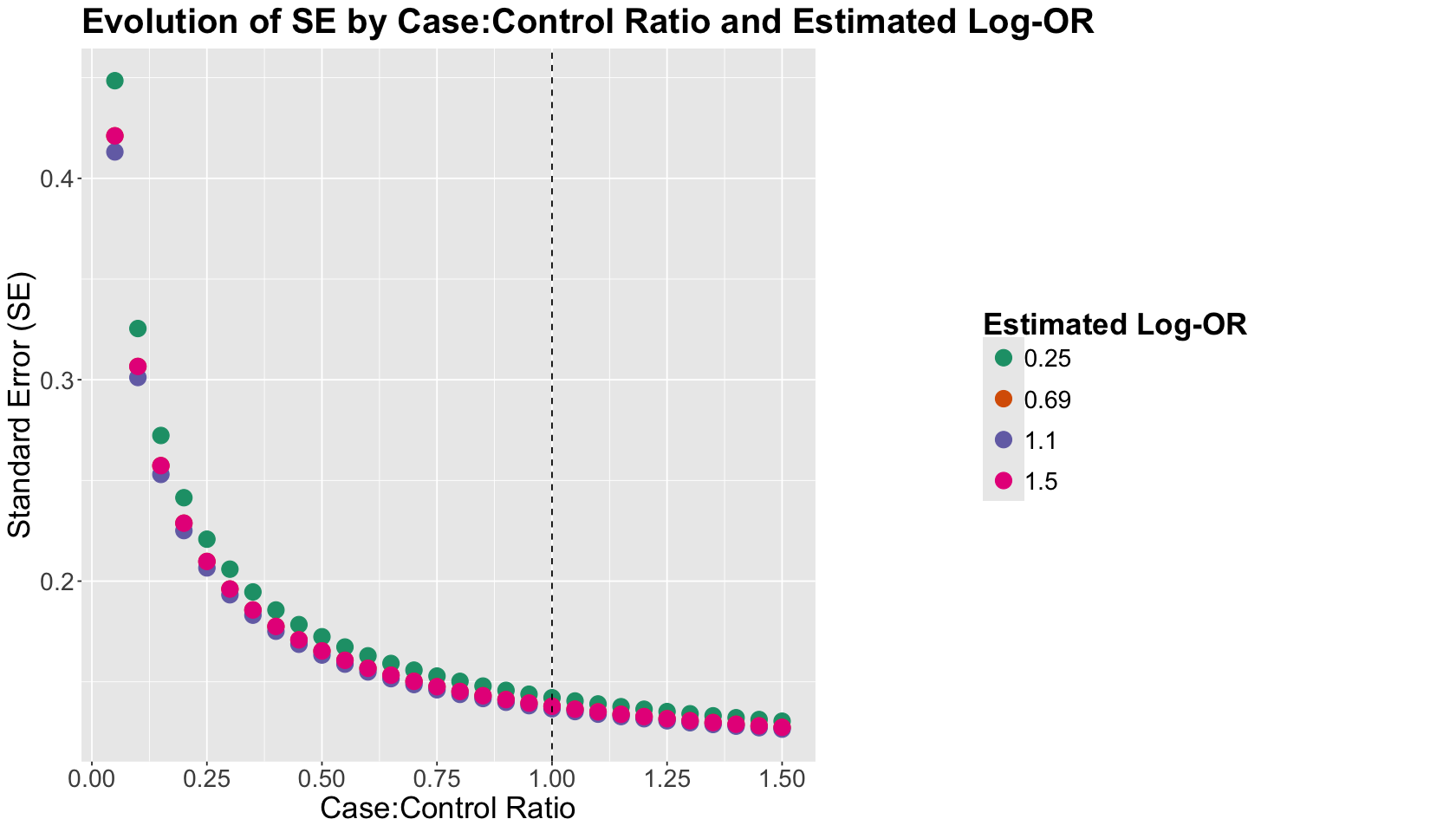
../_images/d1c1c988a650e8023f4e33b5c73df1a66b763c1c46cdbca163be8f405031ba51.png

What is the main takeaway from this plot?

According to the SE behaviour, in populations where the event \(Y = 1\) is rare, we get a more precise estimate of the \(\text{log-OR}\) when we oversample cases and undersample controls. This is even more beneficial in situations where the estimated \(\text{log-OR}\) is low (as shown in our colour scale). Ideally, we might keep the \(\text{Case:Control ratio}\) in \(1\) or slightly above in a CC scheme if \(Y = 1\) is extremely rare.

6. Wrapping Up#

We have learned a new way to assess a given sampling scheme by relying on previously sampled data.
This sampled data would allow building a proxy ground truth so we can run whole simulation studies for each sampling scheme. This proxy ground truth is assumed to be governed by a population regression model.
Note there is a constant tool we use in our simulations: adding random noise.
From the three sampling schemes we explored, CC can provide a boost in accuracy and precision.

Lecture 7 - Observational Data: Different Sampling Schemes

Contents

Lecture 7 - Observational Data: Different Sampling Schemes#

Today’s Learning Objectives#

Loading R Packages#

Previously…#

1. Sampling Schemes in Observational Studies#

1.1. Sampling Assessment Via the Ground Truth#

1.2. Simulation: A Proxy of the Ground Truth#

2. The Western Collaborative Group Study Data#

2.1. Step 1: Use a Relevant Sample Dataset#

2.2. Step 2: Fit a Model#

2.3. Step 3: Simulate a Proxy Ground Truth#

3. Running Three Sampling Schemes Using the Proxy Ground Truth#

3.1. Cross-Sectional Sampling Scheme#

3.2. Case-Control Sampling Scheme#

3.3. Cohort Sampling Scheme#

3.4. When to Use What?#

4. Sampling Scheme Assessment#

4.1 Fitting the Models Using the Three Sampling Schemes#

4.2 Running Simulation Studies Using the Three Sampling Schemes#

5. Looking Further into the Case-Control Scheme#

6. Wrapping Up#

Loading `R` Packages#