Lecture 4: Preprocessing, sklearn Pipeline, sklearn ColumnTrasnsformer

UBC Master of Data Science program, 2023-24

Instructor: Varada Kolhatkar

Imports, announcement, LOs

Imports

import sys
import time

import matplotlib.pyplot as plt

%matplotlib inline
import numpy as np
import pandas as pd
from IPython.display import HTML

sys.path.append(os.path.join(os.path.abspath("."), "code"))

import mglearn
from IPython.display import display
from plotting_functions import *

# Classifiers and regressors
from sklearn.dummy import DummyClassifier, DummyRegressor

# Preprocessing and pipeline
from sklearn.impute import SimpleImputer

# train test split and cross validation
from sklearn.model_selection import cross_val_score, cross_validate, train_test_split
from sklearn.neighbors import KNeighborsClassifier, KNeighborsRegressor
from sklearn.pipeline import Pipeline, make_pipeline
from sklearn.compose import ColumnTransformer, make_column_transformer
from sklearn.preprocessing import (
    MinMaxScaler,
    OneHotEncoder,
    OrdinalEncoder,
    StandardScaler,
)
from sklearn.svm import SVC
from sklearn.tree import DecisionTreeClassifier
from utils import *

pd.set_option("display.max_colwidth", 200)

---------------------------------------------------------------------------
NameError                                 Traceback (most recent call last)
Cell In[1], line 11
      8 import pandas as pd
      9 from IPython.display import HTML
---> 11 sys.path.append(os.path.join(os.path.abspath("."), "code"))
     13 import mglearn
     14 from IPython.display import display

NameError: name 'os' is not defined

Learning outcomes

From this lecture, you will be able to

• explain motivation for preprocessing in supervised machine learning;

• identify when to implement feature transformations such as imputation, scaling, and one-hot encoding in a machine learning model development pipeline;

• use sklearn transformers for applying feature transformations on your dataset;

• discuss golden rule in the context of feature transformations;

• use sklearn.pipeline.Pipeline and sklearn.pipeline.make_pipeline to build a preliminary machine learning pipeline.

• use ColumnTransformer to build all our transformations together into one object and use it with sklearn pipelines;

• define ColumnTransformer where transformers contain more than one steps;

❓❓ Questions for you

(iClicker) Exercise 4.0

iClicker cloud join link: https://join.iclicker.com/DAZZ

Take a guess: In your machine learning project, how much time will you typically spend on data preparation and transformation?

• (A) ~80% of the project time

• (B) ~20% of the project time

• (C) ~50% of the project time

• (D) None. Most of the time will be spent on model building.

The question is adapted from here.

Motivation and big picture [video]

• So far we have seen

  • Three ML models (decision trees, \(k\)-NNs, SVMs with RBF kernel)

  • ML fundamentals (train-validation-test split, cross-validation, the fundamental tradeoff, the golden rule)

• Are we ready to do machine learning on real-world datasets?

  • Very often real-world datasets need preprocessing before we use them to build ML models.

Example: \(k\)-nearest neighbours on the Spotify dataset

• In lab1 you used DecisionTreeClassifier to predict whether the user would like a particular song or not.

• Can we use \(k\)-NN classifier for this task?

• Intuition: To predict whether the user likes a particular song or not (query point)

  • find the songs that are closest to the query point

  • let them vote on the target

  • take the majority vote as the target for the query point

In order to run the code below, you need to download the dataset from Kaggle.

spotify_df = pd.read_csv("data/spotify.csv", index_col=0)
train_df, test_df = train_test_split(spotify_df, test_size=0.20, random_state=123)
X_train, y_train = (
    train_df.drop(columns=["song_title", "artist", "target"]),
    train_df["target"],
)
X_test, y_test = (
    test_df.drop(columns=["song_title", "artist", "target"]),
    test_df["target"],
)

dummy = DummyClassifier(strategy="most_frequent")
scores = cross_validate(dummy, X_train, y_train, return_train_score=True)
print("Mean validation score %0.3f" % (np.mean(scores["test_score"])))
pd.DataFrame(scores)

Mean validation score 0.508

	fit_time	score_time	test_score	train_score
0	0.000613	0.000442	0.507740	0.507752
1	0.000573	0.000582	0.507740	0.507752
2	0.000790	0.000292	0.507740	0.507752
3	0.000378	0.000272	0.506211	0.508133
4	0.000344	0.000242	0.509317	0.507359

knn = KNeighborsClassifier()
scores = cross_validate(knn, X_train, y_train, return_train_score=True)
print("Mean validation score %0.3f" % (np.mean(scores["test_score"])))
pd.DataFrame(scores)

Mean validation score 0.546

	fit_time	score_time	test_score	train_score
0	0.002308	0.008383	0.563467	0.717829
1	0.001740	0.007489	0.535604	0.721705
2	0.001425	0.007203	0.529412	0.708527
3	0.001356	0.007267	0.537267	0.721921
4	0.001408	0.007313	0.562112	0.711077

two_songs = X_train.sample(2, random_state=42)
two_songs

	acousticness	danceability	duration_ms	energy	instrumentalness	key	liveness	loudness	mode	speechiness	tempo	time_signature	valence
842	0.229000	0.494	147893	0.666	0.000057	9	0.0469	-9.743	0	0.0351	140.832	4.0	0.704
654	0.000289	0.771	227143	0.949	0.602000	8	0.5950	-4.712	1	0.1750	111.959	4.0	0.372

euclidean_distances(two_songs)

array([[    0.        , 79250.00543825],
       [79250.00543825,     0.        ]])

Let’s consider only two features: duration_ms and tempo.

two_songs_subset = two_songs[["duration_ms", "tempo"]]
two_songs_subset

	duration_ms	tempo
842	147893	140.832
654	227143	111.959

euclidean_distances(two_songs_subset)

array([[    0.        , 79250.00525962],
       [79250.00525962,     0.        ]])

Do you see any problem?

• The distance is completely dominated by the the features with larger values

• The features with smaller values are being ignored.

• Does it matter?

  • Yes! Scale is based on how data was collected.

  • Features on a smaller scale can be highly informative and there is no good reason to ignore them.

  • We want our model to be robust and not sensitive to the scale.

• Was this a problem for decision trees?

Scaling using scikit-learn’s StandardScaler

• We’ll use scikit-learn’s StandardScaler, which is a transformer.

• Only focus on the syntax for now. We’ll talk about scaling in a bit.

from sklearn.preprocessing import StandardScaler

scaler = StandardScaler()  # create feature trasformer object
scaler.fit(X_train)  # fitting the transformer on the train split
X_train_scaled = scaler.transform(X_train)  # transforming the train split
X_test_scaled = scaler.transform(X_test)  # transforming the test split

X_train # original X_train

	acousticness	danceability	duration_ms	energy	instrumentalness	key	liveness	loudness	mode	speechiness	tempo	time_signature	valence
1505	0.004770	0.585	214740	0.614	0.000155	10	0.0762	-5.594	0	0.0370	114.059	4.0	0.2730
813	0.114000	0.665	216728	0.513	0.303000	0	0.1220	-7.314	1	0.3310	100.344	3.0	0.0373
615	0.030200	0.798	216585	0.481	0.000000	7	0.1280	-10.488	1	0.3140	127.136	4.0	0.6400
319	0.106000	0.912	194040	0.317	0.000208	6	0.0723	-12.719	0	0.0378	99.346	4.0	0.9490
320	0.021100	0.697	236456	0.905	0.893000	6	0.1190	-7.787	0	0.0339	119.977	4.0	0.3110
...	...	...	...	...	...	...	...	...	...	...	...	...	...
2012	0.001060	0.584	274404	0.932	0.002690	1	0.1290	-3.501	1	0.3330	74.976	4.0	0.2110
1346	0.000021	0.535	203500	0.974	0.000149	10	0.2630	-3.566	0	0.1720	116.956	4.0	0.4310
1406	0.503000	0.410	256333	0.648	0.000000	7	0.2190	-4.469	1	0.0362	60.391	4.0	0.3420
1389	0.705000	0.894	222307	0.161	0.003300	4	0.3120	-14.311	1	0.0880	104.968	4.0	0.8180
1534	0.623000	0.470	394920	0.156	0.187000	2	0.1040	-17.036	1	0.0399	118.176	4.0	0.0591

1613 rows × 13 columns

Let’s examine transformed value of the energy feature in the first row.

X_train['energy'].iloc[0] 

0.614

(X_train['energy'].iloc[0] - np.mean(X_train['energy']))/ X_train['energy'].std()

-0.3180174485124284

pd.DataFrame(X_train_scaled, columns=X_train.columns, index=X_train.index).head().round(3)

	acousticness	danceability	duration_ms	energy	instrumentalness	key	liveness	loudness	mode	speechiness	tempo	time_signature	valence
1505	-0.698	-0.195	-0.399	-0.318	-0.492	1.276	-0.738	0.396	-1.281	-0.618	-0.294	0.139	-0.908
813	-0.276	0.296	-0.374	-0.796	0.598	-1.487	-0.439	-0.052	0.781	2.728	-0.803	-3.781	-1.861
615	-0.600	1.111	-0.376	-0.947	-0.493	0.447	-0.400	-0.879	0.781	2.535	0.191	0.139	0.576
319	-0.307	1.809	-0.654	-1.722	-0.492	0.170	-0.763	-1.461	-1.281	-0.609	-0.840	0.139	1.825
320	-0.635	0.492	-0.131	1.057	2.723	0.170	-0.458	-0.176	-1.281	-0.653	-0.074	0.139	-0.754

fit and transform paradigm for transformers

• sklearn uses fit and transform paradigms for feature transformations.

• We fit the transformer on the train split and then transform the train split as well as the test split.

• We apply the same transformations on the test split.

sklearn API summary: estimators

Suppose model is a classification or regression model.

model.fit(X_train, y_train)
X_train_predictions = model.predict(X_train)
X_test_predictions = model.predict(X_test)

sklearn API summary: transformers

Suppose transformer is a transformer used to change the input representation, for example, to tackle missing values or to scales numeric features.

transformer.fit(X_train, [y_train])
X_train_transformed = transformer.transform(X_train)
X_test_transformed = transformer.transform(X_test)

• You can pass y_train in fit but it’s usually ignored. It allows you to pass it just to be consistent with usual usage of sklearn’s fit method.

• You can also carry out fitting and transforming in one call using fit_transform. But be mindful to use it only on the train split and not on the test split.

• Do you expect DummyClassifier results to change after scaling the data?

• Let’s check whether scaling makes any difference for \(k\)-NNs.

knn_unscaled = KNeighborsClassifier()
knn_unscaled.fit(X_train, y_train)
print("Train score: %0.3f" % (knn_unscaled.score(X_train, y_train)))
print("Test score: %0.3f" % (knn_unscaled.score(X_test, y_test)))

Train score: 0.726
Test score: 0.552

knn_scaled = KNeighborsClassifier()
knn_scaled.fit(X_train_scaled, y_train)
print("Train score: %0.3f" % (knn_scaled.score(X_train_scaled, y_train)))
print("Test score: %0.3f" % (knn_scaled.score(X_test_scaled, y_test)))

Train score: 0.798
Test score: 0.686

• The scores with scaled data are better compared to the unscaled data in case of \(k\)-NNs.

• I am not carrying out cross-validation here for a reason that we’ll look into soon.

• Note that I am a bit sloppy here and using the test set several times for teaching purposes. But when you build an ML pipeline, please do assessment on the test set only once.

Common preprocessing techniques

Some commonly performed feature transformation include:

• Imputation: Tackling missing values

• Scaling: Scaling of numeric features

• One-hot encoding: Tackling categorical variables

We can have one lecture on each of them! In this lesson our goal is to getting familiar with them so that we can use them to build ML pipelines.

In the next part of this lecture, we’ll build an ML pipeline using California housing prices regression dataset. In the process, we will talk about different feature transformations and how can we apply them so that we do not violate the golden rule.

Imputation and scaling [video]

Dataset, splitting, and baseline

We’ll be working on California housing prices regression dataset to demonstrate these feature transformation techniques. The task is to predict median house values in Californian districts, given a number of features from these districts. If you are running the notebook on your own, you’ll have to download the data and put it in the data directory.

housing_df = pd.read_csv("data/housing.csv")
train_df, test_df = train_test_split(housing_df, test_size=0.1, random_state=123)

train_df.head()

	longitude	latitude	housing_median_age	total_rooms	total_bedrooms	population	households	median_income	median_house_value	ocean_proximity
6051	-117.75	34.04	22.0	2948.0	636.0	2600.0	602.0	3.1250	113600.0	INLAND
20113	-119.57	37.94	17.0	346.0	130.0	51.0	20.0	3.4861	137500.0	INLAND
14289	-117.13	32.74	46.0	3355.0	768.0	1457.0	708.0	2.6604	170100.0	NEAR OCEAN
13665	-117.31	34.02	18.0	1634.0	274.0	899.0	285.0	5.2139	129300.0	INLAND
14471	-117.23	32.88	18.0	5566.0	1465.0	6303.0	1458.0	1.8580	205000.0	NEAR OCEAN

Some column values are mean/median but some are not.

Let’s add some new features to the dataset which could help predicting the target: median_house_value.

train_df = train_df.assign(
    rooms_per_household=train_df["total_rooms"] / train_df["households"]
)
test_df = test_df.assign(
    rooms_per_household=test_df["total_rooms"] / test_df["households"]
)

train_df = train_df.assign(
    bedrooms_per_household=train_df["total_bedrooms"] / train_df["households"]
)
test_df = test_df.assign(
    bedrooms_per_household=test_df["total_bedrooms"] / test_df["households"]
)

train_df = train_df.assign(
    population_per_household=train_df["population"] / train_df["households"]
)
test_df = test_df.assign(
    population_per_household=test_df["population"] / test_df["households"]
)

train_df.head()

	longitude	latitude	housing_median_age	total_rooms	total_bedrooms	population	households	median_income	median_house_value	ocean_proximity	rooms_per_household	bedrooms_per_household	population_per_household
6051	-117.75	34.04	22.0	2948.0	636.0	2600.0	602.0	3.1250	113600.0	INLAND	4.897010	1.056478	4.318937
20113	-119.57	37.94	17.0	346.0	130.0	51.0	20.0	3.4861	137500.0	INLAND	17.300000	6.500000	2.550000
14289	-117.13	32.74	46.0	3355.0	768.0	1457.0	708.0	2.6604	170100.0	NEAR OCEAN	4.738701	1.084746	2.057910
13665	-117.31	34.02	18.0	1634.0	274.0	899.0	285.0	5.2139	129300.0	INLAND	5.733333	0.961404	3.154386
14471	-117.23	32.88	18.0	5566.0	1465.0	6303.0	1458.0	1.8580	205000.0	NEAR OCEAN	3.817558	1.004801	4.323045

train_df = train_df.drop(columns = ['population', 'total_rooms', 'total_bedrooms'])
test_df =  test_df.drop(columns = ['population', 'total_rooms', 'total_bedrooms'])

When is it OK to do things before splitting?

• Here it would have been OK to add new features before splitting because we are not using any global information in the data but only looking at one row at a time.

• But just to be safe and to avoid accidentally breaking the golden rule, it’s better to do it after splitting.

• Question: Should we remove total_rooms, total_bedrooms, and population columns?

  • Probably. But I am keeping them in this lecture. You could experiment with removing them and examine whether results change.

EDA

train_df.head()

	longitude	latitude	housing_median_age	households	median_income	median_house_value	ocean_proximity	rooms_per_household	bedrooms_per_household	population_per_household
6051	-117.75	34.04	22.0	602.0	3.1250	113600.0	INLAND	4.897010	1.056478	4.318937
20113	-119.57	37.94	17.0	20.0	3.4861	137500.0	INLAND	17.300000	6.500000	2.550000
14289	-117.13	32.74	46.0	708.0	2.6604	170100.0	NEAR OCEAN	4.738701	1.084746	2.057910
13665	-117.31	34.02	18.0	285.0	5.2139	129300.0	INLAND	5.733333	0.961404	3.154386
14471	-117.23	32.88	18.0	1458.0	1.8580	205000.0	NEAR OCEAN	3.817558	1.004801	4.323045

The feature scales are quite different.

train_df.info()

<class 'pandas.core.frame.DataFrame'>
Index: 18576 entries, 6051 to 19966
Data columns (total 10 columns):
 #   Column                    Non-Null Count  Dtype  
---  ------                    --------------  -----  
 0   longitude                 18576 non-null  float64
 1   latitude                  18576 non-null  float64
 2   housing_median_age        18576 non-null  float64
 3   households                18576 non-null  float64
 4   median_income             18576 non-null  float64
 5   median_house_value        18576 non-null  float64
 6   ocean_proximity           18576 non-null  object 
 7   rooms_per_household       18576 non-null  float64
 8   bedrooms_per_household    18391 non-null  float64
 9   population_per_household  18576 non-null  float64
dtypes: float64(9), object(1)
memory usage: 1.6+ MB

We have one categorical feature and all other features are numeric features.

train_df.describe()

	longitude	latitude	housing_median_age	households	median_income	median_house_value	rooms_per_household	bedrooms_per_household	population_per_household
count	18576.000000	18576.000000	18576.000000	18576.000000	18576.000000	18576.000000	18576.000000	18391.000000	18576.000000
mean	-119.565888	35.627966	28.622255	500.061100	3.862552	206292.067991	5.426067	1.097516	3.052349
std	1.999622	2.134658	12.588307	383.044313	1.892491	115083.856175	2.512319	0.486266	10.020873
min	-124.350000	32.540000	1.000000	1.000000	0.499900	14999.000000	0.846154	0.333333	0.692308
25%	-121.790000	33.930000	18.000000	280.000000	2.560225	119400.000000	4.439360	1.005888	2.430323
50%	-118.490000	34.250000	29.000000	410.000000	3.527500	179300.000000	5.226415	1.048860	2.818868
75%	-118.010000	37.710000	37.000000	606.000000	4.736900	263600.000000	6.051620	1.099723	3.283921
max	-114.310000	41.950000	52.000000	6082.000000	15.000100	500001.000000	141.909091	34.066667	1243.333333

• Seems like total_bedrooms column has some missing values.

• This must have affected our new feature bedrooms_per_household as well.

housing_df["total_bedrooms"].isnull().sum()

207

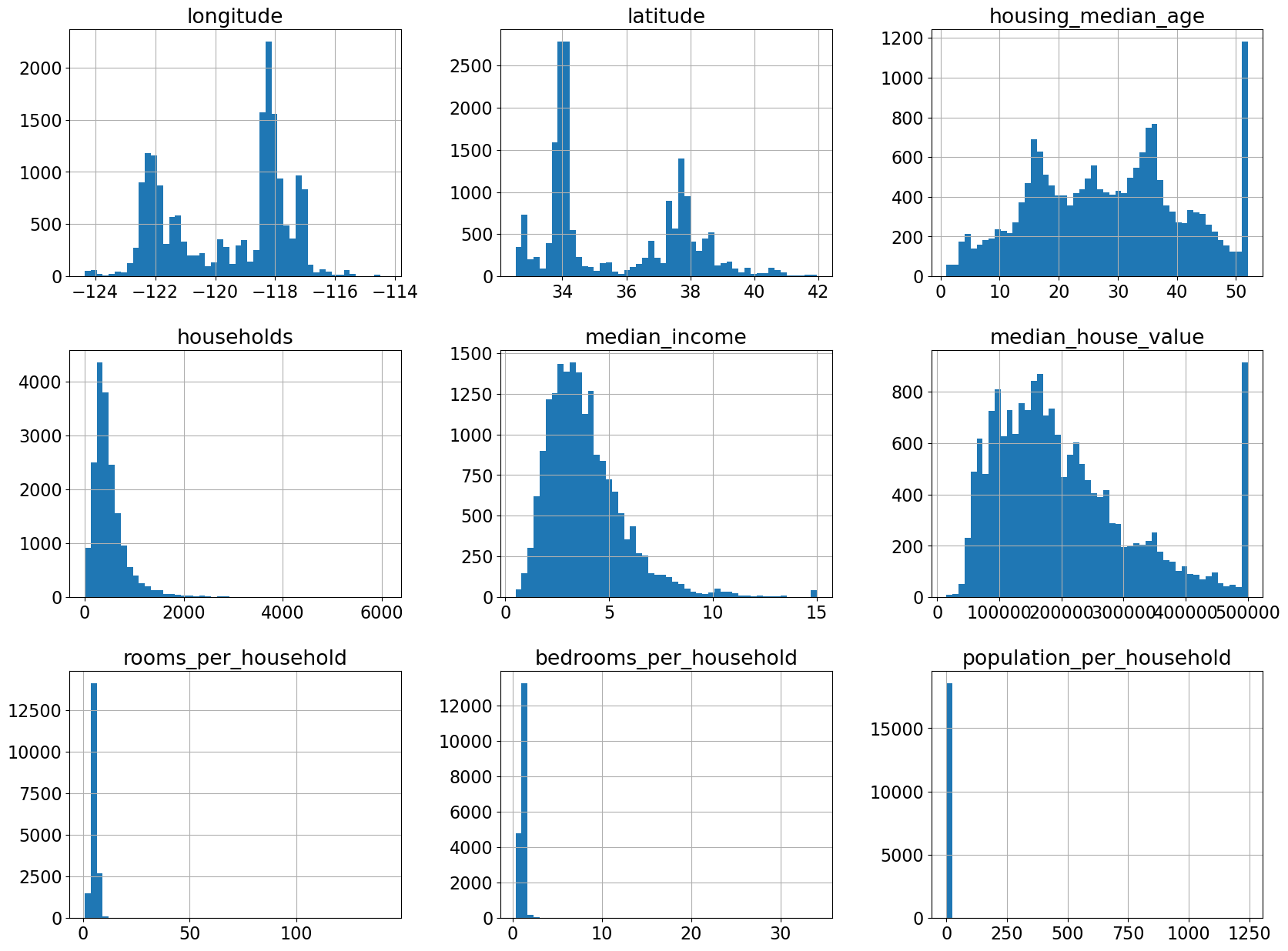
## (optional)
train_df.hist(bins=50, figsize=(20, 15));

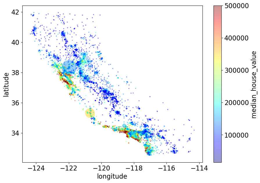
## (optional)
train_df.plot(
    kind="scatter",
    x="longitude",
    y="latitude",
    alpha=0.4,
    s=train_df["population_per_household"],
    figsize=(10, 7),
    c="median_house_value",
    cmap=plt.get_cmap("jet"),
    colorbar=True,
    sharex=False,
);

What all transformations we need to apply on the dataset?

Here is what we see from the EDA.

• Some missing values in total_bedrooms column

• Scales are quite different across columns.

• Categorical variable ocean_proximity

Read about preprocessing techniques implemented in scikit-learn.

# We are droping the categorical variable ocean_proximity for now. We'll come back to it in a bit.
X_train = train_df.drop(columns=["median_house_value", "ocean_proximity"])
y_train = train_df["median_house_value"]

X_test = test_df.drop(columns=["median_house_value", "ocean_proximity"])
y_test = test_df["median_house_value"]

Let’s first run our baseline model DummyRegressor

results_dict = {}  # dictionary to store our results for different models

def mean_std_cross_val_scores(model, X_train, y_train, **kwargs):
    """
    Returns mean and std of cross validation

    Parameters
    ----------
    model :
        scikit-learn model
    X_train : numpy array or pandas DataFrame
        X in the training data
    y_train :
        y in the training data

    Returns
    ----------
        pandas Series with mean scores from cross_validation
    """

    scores = cross_validate(model, X_train, y_train, **kwargs)

    mean_scores = pd.DataFrame(scores).mean()
    std_scores = pd.DataFrame(scores).std()
    out_col = []

    for i in range(len(mean_scores)):
        out_col.append((f"%0.3f (+/- %0.3f)" % (mean_scores.iloc[i], std_scores.iloc[i])))

    return pd.Series(data=out_col, index=mean_scores.index)

dummy = DummyRegressor(strategy="median")
results_dict["dummy"] = mean_std_cross_val_scores(
    dummy, X_train, y_train, return_train_score=True
)

pd.DataFrame(results_dict)

	dummy
fit_time	0.001 (+/- 0.000)
score_time	0.000 (+/- 0.000)
test_score	-0.055 (+/- 0.012)
train_score	-0.055 (+/- 0.001)

Imputation

X_train

	longitude	latitude	housing_median_age	households	median_income	rooms_per_household	bedrooms_per_household	population_per_household
6051	-117.75	34.04	22.0	602.0	3.1250	4.897010	1.056478	4.318937
20113	-119.57	37.94	17.0	20.0	3.4861	17.300000	6.500000	2.550000
14289	-117.13	32.74	46.0	708.0	2.6604	4.738701	1.084746	2.057910
13665	-117.31	34.02	18.0	285.0	5.2139	5.733333	0.961404	3.154386
14471	-117.23	32.88	18.0	1458.0	1.8580	3.817558	1.004801	4.323045
...	...	...	...	...	...	...	...	...
7763	-118.10	33.91	36.0	130.0	3.6389	5.584615	NaN	3.769231
15377	-117.24	33.37	14.0	779.0	4.5391	6.016688	1.017972	3.127086
17730	-121.76	37.33	5.0	697.0	5.6306	5.958393	1.031564	3.493544
15725	-122.44	37.78	44.0	326.0	3.8750	4.739264	1.024540	1.720859
19966	-119.08	36.21	20.0	348.0	2.5156	5.491379	1.117816	3.566092

18576 rows × 8 columns

# knn = KNeighborsRegressor()
# knn.fit(X_train, y_train)

What’s the problem?

ValueError: Input contains NaN, infinity or a value too large for dtype('float64').

• The classifier is not able to deal with missing values (NaNs).

• What are possible ways to deal with the problem?

  • Delete the rows?

  • Replace them with some reasonable values?

• SimpleImputer is a transformer in sklearn to deal with this problem. For example,

  • You can impute missing values in categorical columns with the most frequent value.

  • You can impute the missing values in numeric columns with the mean or median of the column.

X_train.sort_values("bedrooms_per_household")

	longitude	latitude	housing_median_age	households	median_income	rooms_per_household	bedrooms_per_household	population_per_household
20248	-119.23	34.25	28.0	9.0	8.0000	2.888889	0.333333	3.222222
12649	-121.47	38.51	52.0	9.0	3.6250	2.222222	0.444444	8.222222
3125	-117.76	35.22	4.0	6.0	1.6250	3.000000	0.500000	1.333333
12138	-117.22	33.87	16.0	14.0	2.6250	4.000000	0.500000	2.785714
8219	-118.21	33.79	33.0	36.0	4.5938	0.888889	0.500000	2.666667
...	...	...	...	...	...	...	...	...
4591	-118.28	34.06	42.0	1179.0	1.2254	2.096692	NaN	3.218830
19485	-120.98	37.66	10.0	255.0	0.9336	3.662745	NaN	1.572549
6962	-118.05	33.99	38.0	357.0	3.7328	4.535014	NaN	2.481793
14970	-117.01	32.74	31.0	677.0	2.6973	5.129985	NaN	3.098966
7763	-118.10	33.91	36.0	130.0	3.6389	5.584615	NaN	3.769231

18576 rows × 8 columns

X_train.shape
X_test.shape

(2064, 8)

imputer = SimpleImputer(strategy="median")
imputer.fit(X_train)
X_train_imp = imputer.transform(X_train)
X_test_imp = imputer.transform(X_test)

• Let’s check whether the NaN values have been replaced or not

• Note that imputer.transform returns an numpy array and not a dataframe

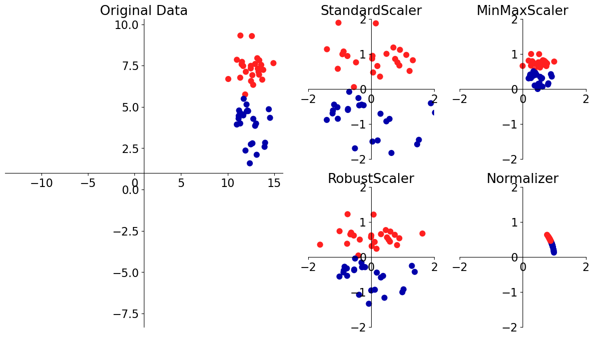
Scaling

• This problem affects a large number of ML methods.

• A number of approaches to this problem. We are going to look into two most popular one.

Approach	What it does	How to update \(X\) (but see below!)	sklearn implementation
standardization	sets sample mean to \(0\), s.d. to \(1\)	X -= np.mean(X,axis=0) X /=  np.std(X,axis=0)	StandardScaler()

There are all sorts of articles on this; see, e.g. here and here.

# [source](https://amueller.github.io/COMS4995-s19/slides/aml-05-preprocessing/#8)
mglearn.plots.plot_scaling()

from sklearn.preprocessing import MinMaxScaler, StandardScaler

scaler = StandardScaler()
X_train_scaled = scaler.fit_transform(X_train_imp)
X_test_scaled = scaler.transform(X_test_imp)
pd.DataFrame(X_train_scaled, columns=X_train.columns)

	longitude	latitude	housing_median_age	households	median_income	rooms_per_household	bedrooms_per_household	population_per_household
0	0.908140	-0.743917	-0.526078	0.266135	-0.389736	-0.210591	-0.083813	0.126398
1	-0.002057	1.083123	-0.923283	-1.253312	-0.198924	4.726412	11.166631	-0.050132
2	1.218207	-1.352930	1.380504	0.542873	-0.635239	-0.273606	-0.025391	-0.099240
3	1.128188	-0.753286	-0.843842	-0.561467	0.714077	0.122307	-0.280310	0.010183
4	1.168196	-1.287344	-0.843842	2.500924	-1.059242	-0.640266	-0.190617	0.126808
...	...	...	...	...	...	...	...	...
18571	0.733102	-0.804818	0.586095	-0.966131	-0.118182	0.063110	-0.099558	0.071541
18572	1.163195	-1.057793	-1.161606	0.728235	0.357500	0.235096	-0.163397	0.007458
18573	-1.097293	0.797355	-1.876574	0.514155	0.934269	0.211892	-0.135305	0.044029
18574	-1.437367	1.008167	1.221622	-0.454427	0.006578	-0.273382	-0.149822	-0.132875
18575	0.242996	0.272667	-0.684960	-0.396991	-0.711754	0.025998	0.042957	0.051269

18576 rows × 8 columns

knn = KNeighborsRegressor()
knn.fit(X_train_scaled, y_train)
knn.score(X_train_scaled, y_train)

0.7978563117812038

• Big difference in the KNN training performance after scaling the data.

• But we saw last week that training score doesn’t tell us much. We should look at the cross-validation score.

❓❓ Questions for you

(iClicker) Exercise 4.1

iClicker cloud join link: https://join.iclicker.com/DAZZ

Select all of the following statements which are TRUE.

• (A) StandardScaler ensures a fixed range (i.e., minimum and maximum values) for the features.

• (B) StandardScaler calculates mean and standard deviation for each feature separately.

• (C) In general, it’s a good idea to apply scaling on numeric features before training \(k\)-NN or SVM RBF models.

• (D) The transformed feature values might be hard to interpret for humans.

• (E) After applying SimpleImputer The transformed data has a different shape than the original data.

V’s Solutions!

B, C, D

Cross validation with already preprocessed data (for class discussion)

knn = KNeighborsRegressor()

scaler = StandardScaler()
scaler.fit(X_train_imp)

X_train_scaled = scaler.transform(X_train_imp)
X_test_scaled = scaler.transform(X_test_imp)
scores = cross_validate(knn, X_train_scaled, y_train, return_train_score=True)
pd.DataFrame(scores)

	fit_time	score_time	test_score	train_score
0	0.007331	0.135313	0.696373	0.794236
1	0.007380	0.120086	0.684447	0.791467
2	0.007231	0.130690	0.695532	0.789436
3	0.007182	0.132624	0.679478	0.793243
4	0.007233	0.081421	0.680657	0.794820

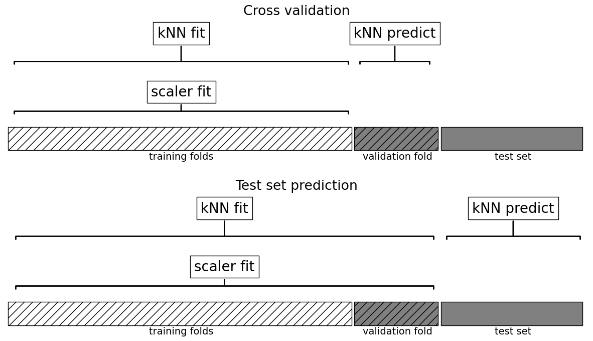
• Is there anything wrong in this methodology? Are we breaking the golden rule here?

plot_improper_processing("kNN")

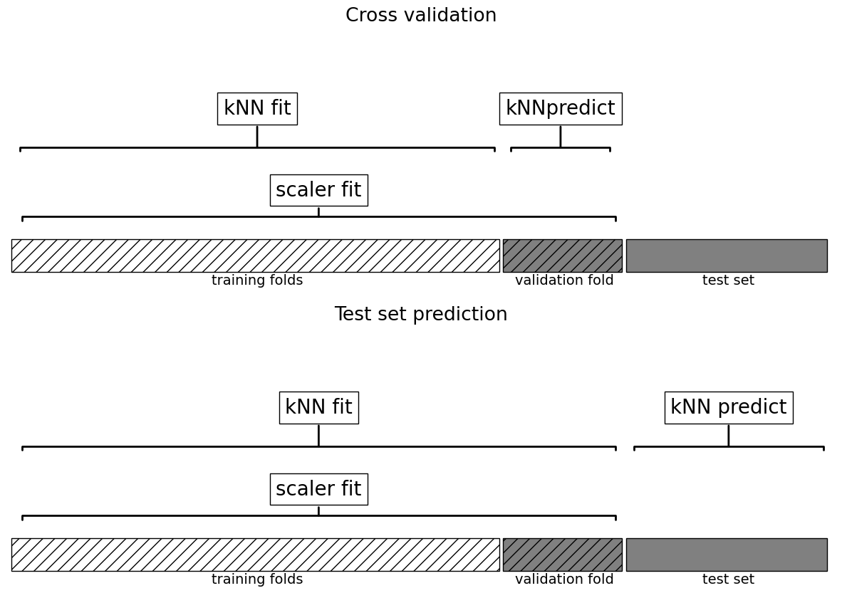
plot_proper_processing("kNN")

Feature transformations and the golden rule

How to carry out cross-validation?

• Last week we saw that cross validation is a better way to get a realistic assessment of the model.

• Let’s try cross-validation with transformed data.

knn = KNeighborsRegressor()

imp = SimpleImputer()
imp.fit(X_train)
X_train_imp = imp.transform(X_train)
X_test_imp = imp.transform(X_test)
scaler = StandardScaler()
scaler.fit(X_train_imp)
X_train_scaled = scaler.transform(X_train_imp)
X_test_scaled = scaler.transform(X_test_imp)
scores = cross_validate(knn, X_train_scaled, y_train, return_train_score=True)
pd.DataFrame(scores)

	fit_time	score_time	test_score	train_score
0	0.008406	0.143026	0.696366	0.794493
1	0.007316	0.122274	0.683602	0.791381
2	0.007279	0.130698	0.695518	0.789231
3	0.007429	0.133527	0.679243	0.793318
4	0.007418	0.081750	0.680758	0.794787

• Do you see any problem here?

• Are we applying fit_transform on train portion and transform on validation portion in each fold?

  • Here you might be allowing information from the validation set to leak into the training step.

• You need to apply the SAME preprocessing steps to train/validation.

• With many different transformations and cross validation the code gets unwieldy very quickly.

• Likely to make mistakes and “leak” information.

• In these examples our test accuracies look fine, but our methodology is flawed.

• Implications can be significant in practice!

Pipelines

Can we do this in a more elegant and organized way?

• YES!! Using scikit-learn Pipeline.

• scikit-learn Pipeline allows you to define a “pipeline” of transformers with a final estimator.

Let’s combine the preprocessing and model with pipeline

### Simple example of a pipeline
from sklearn.pipeline import Pipeline

pipe = Pipeline(
    steps=[
        ("imputer", SimpleImputer(strategy="median")),
        ("scaler", StandardScaler()),
        ("regressor", KNeighborsRegressor()),
    ]
)

• Syntax: pass in a list of steps.

• The last step should be a model/classifier/regressor.

• All the earlier steps should be transformers.

Alternative and more compact syntax: make_pipeline

• Shorthand for Pipeline constructor

• Does not permit naming steps

• Instead the names of steps are set to lowercase of their types automatically; StandardScaler() would be named as standardscaler

from sklearn.pipeline import make_pipeline

pipe = make_pipeline(
    SimpleImputer(strategy="median"), StandardScaler(), KNeighborsRegressor()
)

pipe.fit(X_train, y_train)

Pipeline(steps=[('simpleimputer', SimpleImputer(strategy='median')),
                ('standardscaler', StandardScaler()),
                ('kneighborsregressor', KNeighborsRegressor())])

In a Jupyter environment, please rerun this cell to show the HTML representation or trust the notebook.
On GitHub, the HTML representation is unable to render, please try loading this page with nbviewer.org.

• Note that we are passing X_train and not the imputed or scaled data here.

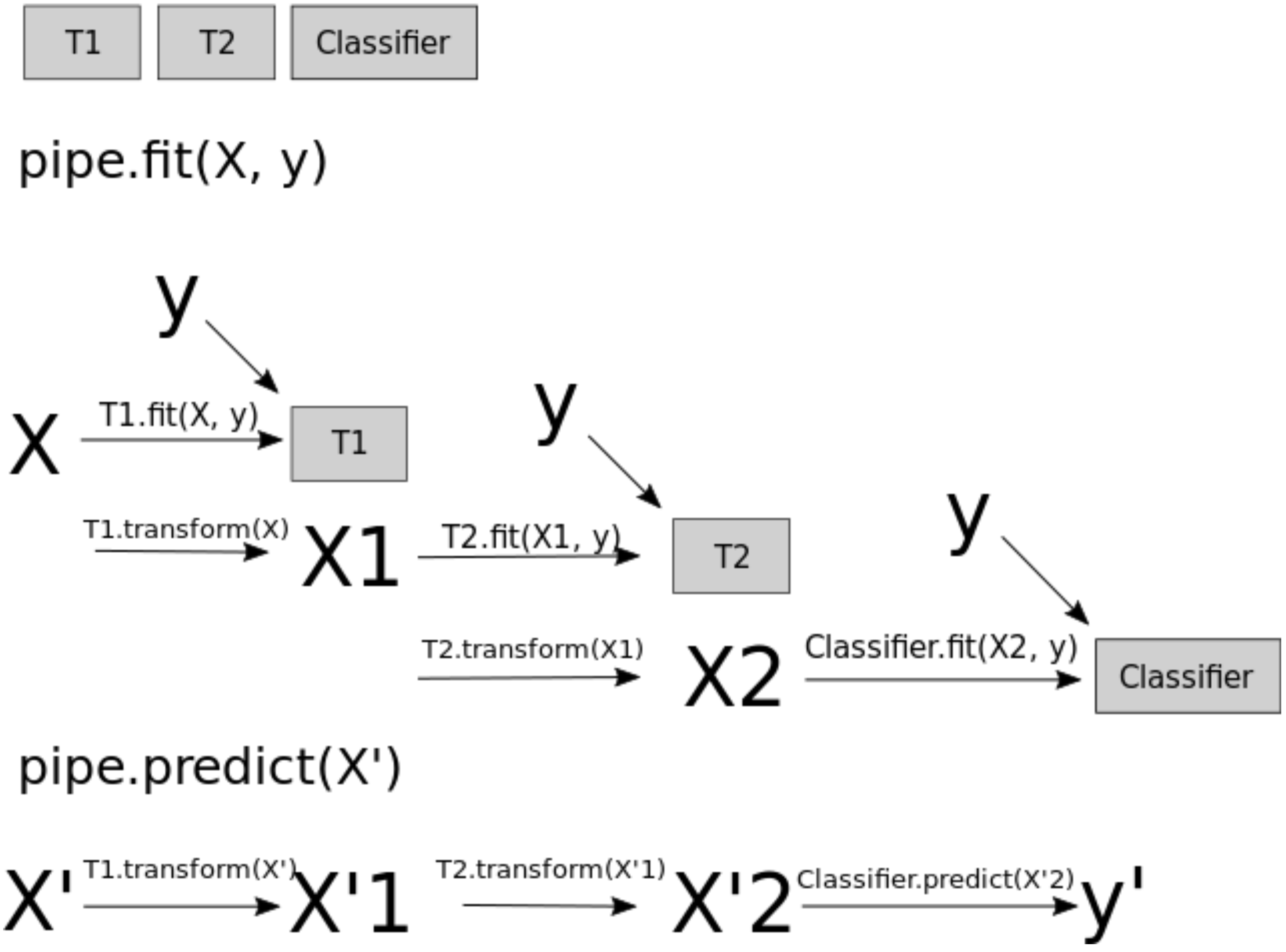
When you call fit on the pipeline, it carries out the following steps:

• Fit SimpleImputer on X_train

• Transform X_train using the fit SimpleImputer to create X_train_imp

• Fit StandardScaler on X_train_imp

• Transform X_train_imp using the fit StandardScaler to create X_train_imp_scaled

• Fit the model (KNeighborsRegressor in our case) on X_train_imp_scaled

pipe.predict(X_train)

array([126500., 117380., 187700., ..., 259500., 308120.,  60860.])

Note that we are passing original data to predict as well. This time the pipeline is carrying out following steps:

• Transform X_train using the fit SimpleImputer to create X_train_imp

• Transform X_train_imp using the fit StandardScaler to create X_train_imp_scaled

• Predict using the fit model (KNeighborsRegressor in our case) on X_train_imp_scaled.

Source

Let’s try cross-validation with our pipeline

results_dict["imp + scaling + knn"] = mean_std_cross_val_scores(
    pipe, X_train, y_train, return_train_score=True
)
pd.DataFrame(results_dict).T

	fit_time	score_time	test_score	train_score
dummy	0.001 (+/- 0.000)	0.000 (+/- 0.000)	-0.055 (+/- 0.012)	-0.055 (+/- 0.001)
imp + scaling + knn	0.018 (+/- 0.001)	0.129 (+/- 0.013)	0.693 (+/- 0.014)	0.797 (+/- 0.015)

Using a Pipeline takes care of applying the fit_transform on the train portion and only transform on the validation portion in each fold.

Break (5 min)

Categorical features [video]

• Recall that we had dropped the categorical feature ocean_proximity feature from the dataframe. But it could potentially be a useful feature in this task.

• Let’s create our X_train and and X_test again by keeping the feature in the data.

X_train

	longitude	latitude	housing_median_age	households	median_income	rooms_per_household	bedrooms_per_household	population_per_household
6051	-117.75	34.04	22.0	602.0	3.1250	4.897010	1.056478	4.318937
20113	-119.57	37.94	17.0	20.0	3.4861	17.300000	6.500000	2.550000
14289	-117.13	32.74	46.0	708.0	2.6604	4.738701	1.084746	2.057910
13665	-117.31	34.02	18.0	285.0	5.2139	5.733333	0.961404	3.154386
14471	-117.23	32.88	18.0	1458.0	1.8580	3.817558	1.004801	4.323045
...	...	...	...	...	...	...	...	...
7763	-118.10	33.91	36.0	130.0	3.6389	5.584615	NaN	3.769231
15377	-117.24	33.37	14.0	779.0	4.5391	6.016688	1.017972	3.127086
17730	-121.76	37.33	5.0	697.0	5.6306	5.958393	1.031564	3.493544
15725	-122.44	37.78	44.0	326.0	3.8750	4.739264	1.024540	1.720859
19966	-119.08	36.21	20.0	348.0	2.5156	5.491379	1.117816	3.566092

18576 rows × 8 columns

X_train = train_df.drop(columns=["median_house_value"])
y_train = train_df["median_house_value"]

X_test = test_df.drop(columns=["median_house_value"])
y_test = test_df["median_house_value"]

• Let’s try to build a KNeighborRegressor on this data using our pipeline

#pipe.fit(X_train, X_train)

• This failed because we have non-numeric data.

• Imagine how \(k\)-NN would calculate distances when you have non-numeric features.

Can we use this feature in the model?

• In scikit-learn, most algorithms require numeric inputs.

• Decision trees could theoretically work with categorical features.

  • However, the sklearn implementation does not support this.

What are the options?

• Drop the column (not recommended)

  • If you know that the column is not relevant to the target in any way you may drop it.

• We can transform categorical features to numeric ones so that we can use them in the model.

  • Ordinal encoding (occasionally recommended)

  • One-hot encoding (recommended in most cases) (this lecture)

X_toy = pd.DataFrame(
    {
        "language": [
            "English",
            "Vietnamese",
            "English",
            "Mandarin",
            "English",
            "English",
            "Mandarin",
            "English",
            "Vietnamese",
            "Mandarin",
            "French",
            "Spanish",
            "Mandarin",
            "Hindi",
        ]
    }
)
X_toy

	language
0	English
1	Vietnamese
2	English
3	Mandarin
4	English
5	English
6	Mandarin
7	English
8	Vietnamese
9	Mandarin
10	French
11	Spanish
12	Mandarin
13	Hindi

Ordinal encoding (occasionally recommended)

• Here we simply assign an integer to each of our unique categorical labels.

• We can use sklearn’s OrdinalEncoder.

from sklearn.preprocessing import OrdinalEncoder

enc = OrdinalEncoder()
enc.fit(X_toy)
X_toy_ord = enc.transform(X_toy)
df = pd.DataFrame(
    data=X_toy_ord,
    columns=["language_enc"],
    index=X_toy.index,
)
pd.concat([X_toy, df], axis=1)

	language	language_enc
0	English	0.0
1	Vietnamese	5.0
2	English	0.0
3	Mandarin	3.0
4	English	0.0
5	English	0.0
6	Mandarin	3.0
7	English	0.0
8	Vietnamese	5.0
9	Mandarin	3.0
10	French	1.0
11	Spanish	4.0
12	Mandarin	3.0
13	Hindi	2.0

What’s the problem with this approach?

• We have imposed ordinality on the categorical data.

• For example, imagine when you are calculating distances. Is it fair to say that French and Hindi are closer than French and Spanish?

• In general, label encoding is useful if there is ordinality in your data and capturing it is important for your problem, e.g., [cold, warm, hot].

One-hot encoding (OHE)

• Create new binary columns to represent our categories.

• If we have \(c\) categories in our column.

  • We create \(c\) new binary columns to represent those categories.

• Example: Imagine a language column which has the information on whether you

• We can use sklearn’s OneHotEncoder to do so.

Note

One-hot encoding is called one-hot because only one of the newly created features is 1 for each data point.

from sklearn.preprocessing import OneHotEncoder

enc = OneHotEncoder(handle_unknown="ignore", sparse_output=False)
enc.fit(X_toy)
X_toy_ohe = enc.transform(X_toy)
pd.DataFrame(
    data=X_toy_ohe,
    columns=enc.get_feature_names_out(["language"]),
    index=X_toy.index,
)

	language_English	language_French	language_Hindi	language_Mandarin	language_Spanish	language_Vietnamese
0	1.0	0.0	0.0	0.0	0.0	0.0
1	0.0	0.0	0.0	0.0	0.0	1.0
2	1.0	0.0	0.0	0.0	0.0	0.0
3	0.0	0.0	0.0	1.0	0.0	0.0
4	1.0	0.0	0.0	0.0	0.0	0.0
5	1.0	0.0	0.0	0.0	0.0	0.0
6	0.0	0.0	0.0	1.0	0.0	0.0
7	1.0	0.0	0.0	0.0	0.0	0.0
8	0.0	0.0	0.0	0.0	0.0	1.0
9	0.0	0.0	0.0	1.0	0.0	0.0
10	0.0	1.0	0.0	0.0	0.0	0.0
11	0.0	0.0	0.0	0.0	1.0	0.0
12	0.0	0.0	0.0	1.0	0.0	0.0
13	0.0	0.0	1.0	0.0	0.0	0.0

Let’s do it on our housing data

ohe = OneHotEncoder(sparse_output=False, dtype=int)
ohe.fit(X_train[["ocean_proximity"]])
X_imp_ohe_train = ohe.transform(X_train[["ocean_proximity"]])

• We can look at the new features created using categories_ attribute

ohe.categories_

[array(['<1H OCEAN', 'INLAND', 'ISLAND', 'NEAR BAY', 'NEAR OCEAN'],
       dtype=object)]

transformed_ohe = pd.DataFrame(
    data=X_imp_ohe_train,
    columns=ohe.get_feature_names_out(["ocean_proximity"]),
    index=X_train.index,
)
transformed_ohe

	ocean_proximity_<1H OCEAN	ocean_proximity_INLAND	ocean_proximity_ISLAND	ocean_proximity_NEAR BAY	ocean_proximity_NEAR OCEAN
6051	0	1	0	0	0
20113	0	1	0	0	0
14289	0	0	0	0	1
13665	0	1	0	0	0
14471	0	0	0	0	1
...	...	...	...	...	...
7763	1	0	0	0	0
15377	1	0	0	0	0
17730	1	0	0	0	0
15725	0	0	0	1	0
19966	0	1	0	0	0

18576 rows × 5 columns

See also

One-hot encoded variables are also referred to as dummy variables. You will often see people using get_dummies method of pandas to convert categorical variables into dummy variables. That said, using sklearn’s OneHotEncoder has the advantage of making it easy to treat training and test set in a consistent way.

❓❓ Questions for you

(iClicker) Exercise 4.2

iClicker cloud join link: https://join.iclicker.com/DAZZ

Select all of the following statements which are TRUE.

• (A) You can have scaling of numeric features, one-hot encoding of categorical features, and scikit-learn estimator within a single pipeline.

• (B) Once you have a scikit-learn pipeline object with an estimator as the last step, you can call fit, predict, and score on it.

• (C) You can carry out data splitting within scikit-learn pipeline.

• (D) We have to be careful of the order we put each transformation and model in a pipeline.

• (E) If you call cross_validate with a pipeline object, it will call fit and transform on the training fold and only transform on the validation fold.

V’s Solutions!

B, D, E

Problem: Different transformations on different columns

• How do we put this together with other columns in the data before fitting the regressor?

• Before we fit our regressor, we want to apply different transformations on different columns

  • Numeric columns

    • imputation

    • scaling

  • Categorical columns

    • imputation

    • one-hot encoding

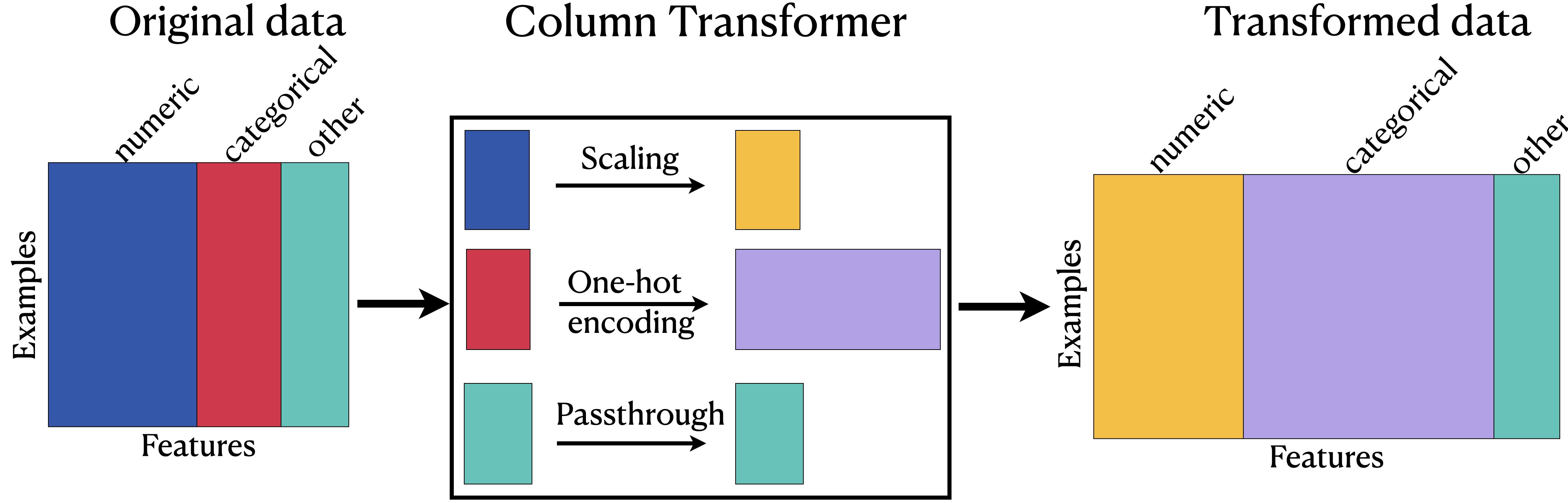
sklearn’s ColumnTransformer

• In most applications, some features are categorical, some are continuous, some are binary, and some are ordinal.

• When we want to develop supervised machine learning pipelines on real-world datasets, very often we want to apply different transformation on different columns.

• Enter sklearn’s ColumnTransformer!!

• Let’s look at a toy example:

df = pd.read_csv("data/quiz2-grade-toy-col-transformer.csv")
df.head()

	enjoy_course	ml_experience	major	class_attendance	university_years	lab1	lab2	lab3	lab4	quiz1	quiz2
0	yes	1	Computer Science	Excellent	3	92	93.0	84	91	92	A+
1	yes	1	Mechanical Engineering	Average	2	94	90.0	80	83	91	not A+
2	yes	0	Mathematics	Poor	3	78	85.0	83	80	80	not A+
3	no	0	Mathematics	Excellent	3	91	NaN	92	91	89	A+
4	yes	0	Psychology	Good	4	77	83.0	90	92	85	A+

df.info()

<class 'pandas.core.frame.DataFrame'>
RangeIndex: 21 entries, 0 to 20
Data columns (total 11 columns):
 #   Column            Non-Null Count  Dtype  
---  ------            --------------  -----  
 0   enjoy_course      21 non-null     object 
 1   ml_experience     21 non-null     int64  
 2   major             21 non-null     object 
 3   class_attendance  21 non-null     object 
 4   university_years  21 non-null     int64  
 5   lab1              21 non-null     int64  
 6   lab2              19 non-null     float64
 7   lab3              21 non-null     int64  
 8   lab4              21 non-null     int64  
 9   quiz1             21 non-null     int64  
 10  quiz2             21 non-null     object 
dtypes: float64(1), int64(6), object(4)
memory usage: 1.9+ KB

Transformations on the toy data

df.head()

	enjoy_course	ml_experience	major	class_attendance	university_years	lab1	lab2	lab3	lab4	quiz1	quiz2
0	yes	1	Computer Science	Excellent	3	92	93.0	84	91	92	A+
1	yes	1	Mechanical Engineering	Average	2	94	90.0	80	83	91	not A+
2	yes	0	Mathematics	Poor	3	78	85.0	83	80	80	not A+
3	no	0	Mathematics	Excellent	3	91	NaN	92	91	89	A+
4	yes	0	Psychology	Good	4	77	83.0	90	92	85	A+

• Scaling on numeric features

• One-hot encoding on the categorical feature major and binary feature enjoy_class

• Ordinal encoding on the ordinal feature class_attendance

• Imputation on the lab2 feature

• None on the ml_experience feature

ColumnTransformer example

Data

X = df.drop(columns=["quiz2"])
y = df["quiz2"]
X.columns

Index(['enjoy_course', 'ml_experience', 'major', 'class_attendance',
       'university_years', 'lab1', 'lab2', 'lab3', 'lab4', 'quiz1'],
      dtype='object')

Identify the transformations we want to apply

X.head()

	enjoy_course	ml_experience	major	class_attendance	university_years	lab1	lab2	lab3	lab4	quiz1
0	yes	1	Computer Science	Excellent	3	92	93.0	84	91	92
1	yes	1	Mechanical Engineering	Average	2	94	90.0	80	83	91
2	yes	0	Mathematics	Poor	3	78	85.0	83	80	80
3	no	0	Mathematics	Excellent	3	91	NaN	92	91	89
4	yes	0	Psychology	Good	4	77	83.0	90	92	85

numeric_feats = ["university_years", "lab1", "lab3", "lab4", "quiz1"]  # apply scaling
categorical_feats = ["major"]  # apply one-hot encoding
passthrough_feats = ["ml_experience"]  # do not apply any transformation
drop_feats = [
    "lab2",
    "class_attendance",
    "enjoy_course",
]  # do not include these features in modeling

For simplicity, let’s only focus on scaling and one-hot encoding first.

Create a column transformer

• Each transformation is specified by a name, a transformer object, and the columns this transformer should be applied to.

from sklearn.compose import ColumnTransformer

ct = ColumnTransformer(
    [
        ("scaling", StandardScaler(), numeric_feats),
        ("onehot", OneHotEncoder(sparse_output=False), categorical_feats),
    ]
)

Convenient make_column_transformer syntax

• Similar to make_pipeline syntax, there is convenient make_column_transformer syntax.

• The syntax automatically names each step based on its class.

• We’ll be mostly using this syntax.

from sklearn.compose import make_column_transformer

ct = make_column_transformer(    
    (StandardScaler(), numeric_feats),  # scaling on numeric features
    ("passthrough", passthrough_feats),  # no transformations on the binary features    
    (OneHotEncoder(), categorical_feats),  # OHE on categorical features
    ("drop", drop_feats),  # drop the drop features
)

ct

ColumnTransformer(transformers=[('standardscaler', StandardScaler(),
                                 ['university_years', 'lab1', 'lab3', 'lab4',
                                  'quiz1']),
                                ('passthrough', 'passthrough',
                                 ['ml_experience']),
                                ('onehotencoder', OneHotEncoder(), ['major']),
                                ('drop', 'drop',
                                 ['lab2', 'class_attendance', 'enjoy_course'])])

In a Jupyter environment, please rerun this cell to show the HTML representation or trust the notebook.
On GitHub, the HTML representation is unable to render, please try loading this page with nbviewer.org.

transformed = ct.fit_transform(X)

• When we fit_transform, each transformer is applied to the specified columns and the result of the transformations are concatenated horizontally.

• A big advantage here is that we build all our transformations together into one object, and that way we’re sure we do the same operations to all splits of the data.

• Otherwise we might, for example, do the OHE on both train and test but forget to scale the test data.

Let’s examine the transformed data

type(transformed[:2])

numpy.ndarray

transformed

array([[-0.09345386,  0.3589134 , -0.21733442,  0.36269995,  0.84002795,
         1.        ,  0.        ,  1.        ,  0.        ,  0.        ,
         0.        ,  0.        ,  0.        ,  0.        ],
       [-1.07471942,  0.59082668, -0.61420598, -0.85597188,  0.71219761,
         1.        ,  0.        ,  0.        ,  0.        ,  0.        ,
         0.        ,  1.        ,  0.        ,  0.        ],
       [-0.09345386, -1.26447953, -0.31655231, -1.31297381, -0.69393613,
         0.        ,  0.        ,  0.        ,  0.        ,  0.        ,
         1.        ,  0.        ,  0.        ,  0.        ],
       [-0.09345386,  0.24295676,  0.57640869,  0.36269995,  0.45653693,
         0.        ,  0.        ,  0.        ,  0.        ,  0.        ,
         1.        ,  0.        ,  0.        ,  0.        ],
       [ 0.8878117 , -1.38043616,  0.37797291,  0.51503393, -0.05478443,
         0.        ,  0.        ,  0.        ,  0.        ,  0.        ,
         0.        ,  0.        ,  0.        ,  1.        ],
       [ 1.86907725, -2.19213263, -1.80482065, -2.22697768, -1.84440919,
         1.        ,  0.        ,  0.        ,  1.        ,  0.        ,
         0.        ,  0.        ,  0.        ,  0.        ],
       [ 0.8878117 , -1.03256625,  0.27875502, -0.09430199,  0.71219761,
         1.        ,  0.        ,  1.        ,  0.        ,  0.        ,
         0.        ,  0.        ,  0.        ,  0.        ],
       [-0.09345386,  0.70678332, -1.70560276, -1.46530779, -1.33308783,
         0.        ,  0.        ,  0.        ,  0.        ,  0.        ,
         0.        ,  1.        ,  0.        ,  0.        ],
       [-1.07471942,  0.93869659,  0.77484447, -1.00830586, -0.69393613,
         0.        ,  0.        ,  0.        ,  0.        ,  1.        ,
         0.        ,  0.        ,  0.        ,  0.        ],
       [ 0.8878117 ,  0.70678332,  0.77484447,  0.81970188, -0.05478443,
         1.        ,  0.        ,  0.        ,  0.        ,  0.        ,
         1.        ,  0.        ,  0.        ,  0.        ],
       [-0.09345386,  1.05465323,  0.87406235,  0.97203586, -0.94959681,
         0.        ,  0.        ,  0.        ,  0.        ,  0.        ,
         0.        ,  0.        ,  0.        ,  1.        ],
       [-2.05598498,  0.70678332,  0.67562658,  0.51503393, -0.05478443,
         1.        ,  0.        ,  0.        ,  0.        ,  0.        ,
         0.        ,  0.        ,  1.        ,  0.        ],
       [-1.07471942,  1.05465323,  0.97328024,  1.58137177,  1.86267067,
         1.        ,  0.        ,  0.        ,  0.        ,  0.        ,
         0.        ,  0.        ,  1.        ,  0.        ],
       [ 0.8878117 ,  0.70678332,  0.97328024,  0.97203586,  1.86267067,
         0.        ,  0.        ,  0.        ,  0.        ,  0.        ,
         0.        ,  1.        ,  0.        ,  0.        ],
       [-0.09345386,  0.70678332,  0.67562658,  0.97203586, -1.97223953,
         0.        ,  0.        ,  0.        ,  0.        ,  0.        ,
         1.        ,  0.        ,  0.        ,  0.        ],
       [-0.09345386,  0.3589134 , -1.90403853,  0.81970188,  0.84002795,
         1.        ,  0.        ,  1.        ,  0.        ,  0.        ,
         0.        ,  0.        ,  0.        ,  0.        ],
       [ 1.86907725, -1.61234944,  0.67562658, -0.39896994, -0.05478443,
         0.        ,  0.        ,  1.        ,  0.        ,  0.        ,
         0.        ,  0.        ,  0.        ,  0.        ],
       [-0.09345386, -0.33682642, -2.10247431, -0.39896994,  0.20087625,
         1.        ,  0.        ,  0.        ,  1.        ,  0.        ,
         0.        ,  0.        ,  0.        ,  0.        ],
       [-1.07471942,  0.24295676,  0.37797291, -0.09430199, -0.43827545,
         1.        ,  1.        ,  0.        ,  0.        ,  0.        ,
         0.        ,  0.        ,  0.        ,  0.        ],
       [-1.07471942, -1.38043616,  0.08031924, -1.16063983,  0.45653693,
         0.        ,  0.        ,  0.        ,  0.        ,  0.        ,
         0.        ,  0.        ,  0.        ,  1.        ],
       [ 0.8878117 ,  0.82273995,  0.57640869,  1.12436984,  0.20087625,
         1.        ,  0.        ,  0.        ,  0.        ,  1.        ,
         0.        ,  0.        ,  0.        ,  0.        ]])

Note

Note that the returned object is not a dataframe. So there are no column names.

Viewing the transformed data as a dataframe

• How can we view our transformed data as a dataframe?

• We are adding more columns.

• So the original columns won’t directly map to the transformed data.

• Let’s create column names for the transformed data.

column_names = (
    numeric_feats
    + passthrough_feats    
    + ct.named_transformers_["onehotencoder"].get_feature_names_out().tolist()
)
column_names

['university_years',
 'lab1',
 'lab3',
 'lab4',
 'quiz1',
 'ml_experience',
 'major_Biology',
 'major_Computer Science',
 'major_Economics',
 'major_Linguistics',
 'major_Mathematics',
 'major_Mechanical Engineering',
 'major_Physics',
 'major_Psychology']

ct.named_transformers_

{'standardscaler': StandardScaler(),
 'passthrough': 'passthrough',
 'onehotencoder': OneHotEncoder(),
 'drop': 'drop'}

Note

Note that the order of the columns in the transformed data depends upon the order of the features we pass to the ColumnTransformer and can be different than the order of the features in the original dataframe.

pd.DataFrame(transformed, columns=column_names)

	university_years	lab1	lab3	lab4	quiz1	ml_experience	major_Biology	major_Computer Science	major_Economics	major_Linguistics	major_Mathematics	major_Mechanical Engineering	major_Physics	major_Psychology
0	-0.093454	0.358913	-0.217334	0.362700	0.840028	1.0	0.0	1.0	0.0	0.0	0.0	0.0	0.0	0.0
1	-1.074719	0.590827	-0.614206	-0.855972	0.712198	1.0	0.0	0.0	0.0	0.0	0.0	1.0	0.0	0.0
2	-0.093454	-1.264480	-0.316552	-1.312974	-0.693936	0.0	0.0	0.0	0.0	0.0	1.0	0.0	0.0	0.0
3	-0.093454	0.242957	0.576409	0.362700	0.456537	0.0	0.0	0.0	0.0	0.0	1.0	0.0	0.0	0.0
4	0.887812	-1.380436	0.377973	0.515034	-0.054784	0.0	0.0	0.0	0.0	0.0	0.0	0.0	0.0	1.0
5	1.869077	-2.192133	-1.804821	-2.226978	-1.844409	1.0	0.0	0.0	1.0	0.0	0.0	0.0	0.0	0.0
6	0.887812	-1.032566	0.278755	-0.094302	0.712198	1.0	0.0	1.0	0.0	0.0	0.0	0.0	0.0	0.0
7	-0.093454	0.706783	-1.705603	-1.465308	-1.333088	0.0	0.0	0.0	0.0	0.0	0.0	1.0	0.0	0.0
8	-1.074719	0.938697	0.774844	-1.008306	-0.693936	0.0	0.0	0.0	0.0	1.0	0.0	0.0	0.0	0.0
9	0.887812	0.706783	0.774844	0.819702	-0.054784	1.0	0.0	0.0	0.0	0.0	1.0	0.0	0.0	0.0
10	-0.093454	1.054653	0.874062	0.972036	-0.949597	0.0	0.0	0.0	0.0	0.0	0.0	0.0	0.0	1.0
11	-2.055985	0.706783	0.675627	0.515034	-0.054784	1.0	0.0	0.0	0.0	0.0	0.0	0.0	1.0	0.0
12	-1.074719	1.054653	0.973280	1.581372	1.862671	1.0	0.0	0.0	0.0	0.0	0.0	0.0	1.0	0.0
13	0.887812	0.706783	0.973280	0.972036	1.862671	0.0	0.0	0.0	0.0	0.0	0.0	1.0	0.0	0.0
14	-0.093454	0.706783	0.675627	0.972036	-1.972240	0.0	0.0	0.0	0.0	0.0	1.0	0.0	0.0	0.0
15	-0.093454	0.358913	-1.904039	0.819702	0.840028	1.0	0.0	1.0	0.0	0.0	0.0	0.0	0.0	0.0
16	1.869077	-1.612349	0.675627	-0.398970	-0.054784	0.0	0.0	1.0	0.0	0.0	0.0	0.0	0.0	0.0
17	-0.093454	-0.336826	-2.102474	-0.398970	0.200876	1.0	0.0	0.0	1.0	0.0	0.0	0.0	0.0	0.0
18	-1.074719	0.242957	0.377973	-0.094302	-0.438275	1.0	1.0	0.0	0.0	0.0	0.0	0.0	0.0	0.0
19	-1.074719	-1.380436	0.080319	-1.160640	0.456537	0.0	0.0	0.0	0.0	0.0	0.0	0.0	0.0	1.0
20	0.887812	0.822740	0.576409	1.124370	0.200876	1.0	0.0	0.0	0.0	1.0	0.0	0.0	0.0	0.0

ColumnTransformer: Transformed data

Adapted from here.

Training models with transformed data

• We can now pass the ColumnTransformer object as a step in a pipeline.

pipe = make_pipeline(ct, SVC())
pipe.fit(X, y)
pipe.predict(X)

array(['A+', 'not A+', 'not A+', 'A+', 'A+', 'not A+', 'A+', 'not A+',
       'not A+', 'A+', 'A+', 'A+', 'A+', 'A+', 'not A+', 'not A+', 'A+',
       'not A+', 'not A+', 'not A+', 'A+'], dtype=object)

pipe

Pipeline(steps=[('columntransformer',
                 ColumnTransformer(transformers=[('standardscaler',
                                                  StandardScaler(),
                                                  ['university_years', 'lab1',
                                                   'lab3', 'lab4', 'quiz1']),
                                                 ('passthrough', 'passthrough',
                                                  ['ml_experience']),
                                                 ('onehotencoder',
                                                  OneHotEncoder(), ['major']),
                                                 ('drop', 'drop',
                                                  ['lab2', 'class_attendance',
                                                   'enjoy_course'])])),
                ('svc', SVC())])

In a Jupyter environment, please rerun this cell to show the HTML representation or trust the notebook.
On GitHub, the HTML representation is unable to render, please try loading this page with nbviewer.org.

Incorporating ordinal feature class_attendance

• The class_attendance column is different than the major column in that there is some ordering of the values.

  • Excellent > Good > Average > poor

X.head()

	enjoy_course	ml_experience	major	class_attendance	university_years	lab1	lab2	lab3	lab4	quiz1
0	yes	1	Computer Science	Excellent	3	92	93.0	84	91	92
1	yes	1	Mechanical Engineering	Average	2	94	90.0	80	83	91
2	yes	0	Mathematics	Poor	3	78	85.0	83	80	80
3	no	0	Mathematics	Excellent	3	91	NaN	92	91	89
4	yes	0	Psychology	Good	4	77	83.0	90	92	85

Let’s try applying OrdinalEncoder on this column.

X_toy = X[["class_attendance"]]
enc = OrdinalEncoder()
enc.fit(X_toy)
X_toy_ord = enc.transform(X_toy)
df = pd.DataFrame(
    data=X_toy_ord,
    columns=["class_attendance_enc"],
    index=X_toy.index,
)

pd.concat([X_toy, df], axis=1).head(10)

	class_attendance	class_attendance_enc
0	Excellent	1.0
1	Average	0.0
2	Poor	3.0
3	Excellent	1.0
4	Good	2.0
5	Good	2.0
6	Excellent	1.0
7	Poor	3.0
8	Average	0.0
9	Average	0.0

• What’s the problem here?

  • The encoder doesn’t know the order.

• We can examine unique categories manually, order them based on our intuitions, and then provide this human knowledge to the transformer.

What are the unique categories of class_attendance?

X_toy["class_attendance"].unique()

array(['Excellent', 'Average', 'Poor', 'Good'], dtype=object)

Let’s order them manually.

class_attendance_levels = ["Poor", "Average", "Good", "Excellent"]

Note

Note that if you use the reverse order of the categories, it wouldn’t matter.

Let’s make sure that we have included all categories in our manual ordering.

assert set(class_attendance_levels) == set(X_toy["class_attendance"].unique())

oe = OrdinalEncoder(categories=[class_attendance_levels], dtype=int)
oe.fit(X_toy[["class_attendance"]])
ca_transformed = oe.transform(X_toy[["class_attendance"]])
df = pd.DataFrame(
    data=ca_transformed, columns=["class_attendance_enc"], index=X_toy.index
)
print(oe.categories_)
pd.concat([X_toy, df], axis=1).head(10)

[array(['Poor', 'Average', 'Good', 'Excellent'], dtype=object)]

	class_attendance	class_attendance_enc
0	Excellent	3
1	Average	1
2	Poor	0
3	Excellent	3
4	Good	2
5	Good	2
6	Excellent	3
7	Poor	0
8	Average	1
9	Average	1

The encoded categories are looking better now!

More than one ordinal columns?

• We can pass the manually ordered categories when we create an OrdinalEncoder object as a list of lists.

• If you have more than one ordinal columns

  • manually create a list of ordered categories for each column

  • pass a list of lists to OrdinalEncoder, where each inner list corresponds to manually created list of ordered categories for a corresponding ordinal column.

Now let’s incorporate ordinal encoding of class_attendance in our column transformer.

X

	enjoy_course	ml_experience	major	class_attendance	university_years	lab1	lab2	lab3	lab4	quiz1
0	yes	1	Computer Science	Excellent	3	92	93.0	84	91	92
1	yes	1	Mechanical Engineering	Average	2	94	90.0	80	83	91
2	yes	0	Mathematics	Poor	3	78	85.0	83	80	80
3	no	0	Mathematics	Excellent	3	91	NaN	92	91	89
4	yes	0	Psychology	Good	4	77	83.0	90	92	85
5	no	1	Economics	Good	5	70	73.0	68	74	71
6	yes	1	Computer Science	Excellent	4	80	88.0	89	88	91
7	no	0	Mechanical Engineering	Poor	3	95	93.0	69	79	75
8	no	0	Linguistics	Average	2	97	90.0	94	82	80
9	yes	1	Mathematics	Average	4	95	82.0	94	94	85
10	yes	0	Psychology	Good	3	98	86.0	95	95	78
11	yes	1	Physics	Average	1	95	88.0	93	92	85
12	yes	1	Physics	Excellent	2	98	96.0	96	99	100
13	yes	0	Mechanical Engineering	Excellent	4	95	94.0	96	95	100
14	no	0	Mathematics	Poor	3	95	90.0	93	95	70
15	no	1	Computer Science	Good	3	92	85.0	67	94	92
16	yes	0	Computer Science	Average	5	75	91.0	93	86	85
17	yes	1	Economics	Average	3	86	89.0	65	86	87
18	no	1	Biology	Good	2	91	NaN	90	88	82
19	no	0	Psychology	Poor	2	77	94.0	87	81	89
20	yes	1	Linguistics	Excellent	4	96	92.0	92	96	87

numeric_feats = [
    "university_years",
    "lab1",
    "lab2",
    "lab3",
    "lab4",
    "quiz1",
]  # apply scaling
categorical_feats = ["major"]  # apply one-hot encoding
ordinal_feats = ["class_attendance"]  # apply ordinal encoding
passthrough_feats = ["ml_experience"]  # do not apply any transformation
drop_feats = ["enjoy_course"]  # do not include these features

ct = make_column_transformer(
    (
        make_pipeline(SimpleImputer(), StandardScaler()),
        numeric_feats,
    ),  # scaling on numeric features
    (
        OrdinalEncoder(categories=[class_attendance_levels], dtype=int),
        ordinal_feats,
    ),  # Ordinal encoding on ordinal features
    ("passthrough", passthrough_feats),  # no transformations on the binary features
    (OneHotEncoder(), categorical_feats),  # OHE on categorical features    
    ("drop", drop_feats),  # drop the drop features
)

ct

ColumnTransformer(transformers=[('pipeline',
                                 Pipeline(steps=[('simpleimputer',
                                                  SimpleImputer()),
                                                 ('standardscaler',
                                                  StandardScaler())]),
                                 ['university_years', 'lab1', 'lab2', 'lab3',
                                  'lab4', 'quiz1']),
                                ('ordinalencoder',
                                 OrdinalEncoder(categories=[['Poor', 'Average',
                                                             'Good',
                                                             'Excellent']],
                                                dtype=<class 'int'>),
                                 ['class_attendance']),
                                ('passthrough', 'passthrough',
                                 ['ml_experience']),
                                ('onehotencoder', OneHotEncoder(), ['major']),
                                ('drop', 'drop', ['enjoy_course'])])

In a Jupyter environment, please rerun this cell to show the HTML representation or trust the notebook.
On GitHub, the HTML representation is unable to render, please try loading this page with nbviewer.org.

X_transformed = ct.fit_transform(X)

column_names = (
    numeric_feats
    + ordinal_feats
    + passthrough_feats    
    + ct.named_transformers_["onehotencoder"].get_feature_names_out().tolist()
)
column_names

['university_years',
 'lab1',
 'lab2',
 'lab3',
 'lab4',
 'quiz1',
 'class_attendance',
 'ml_experience',
 'major_Biology',
 'major_Computer Science',
 'major_Economics',
 'major_Linguistics',
 'major_Mathematics',
 'major_Mechanical Engineering',
 'major_Physics',
 'major_Psychology']

pd.DataFrame(X_transformed, columns=column_names)

	university_years	lab1	lab2	lab3	lab4	quiz1	class_attendance	ml_experience	major_Biology	major_Computer Science	major_Economics	major_Linguistics	major_Mathematics	major_Mechanical Engineering	major_Physics	major_Psychology
0	-0.093454	0.358913	0.893260	-0.217334	0.362700	0.840028	3.0	1.0	0.0	1.0	0.0	0.0	0.0	0.0	0.0	0.0
1	-1.074719	0.590827	0.294251	-0.614206	-0.855972	0.712198	1.0	1.0	0.0	0.0	0.0	0.0	0.0	1.0	0.0	0.0
2	-0.093454	-1.264480	-0.704099	-0.316552	-1.312974	-0.693936	0.0	0.0	0.0	0.0	0.0	0.0	1.0	0.0	0.0	0.0
3	-0.093454	0.242957	0.000000	0.576409	0.362700	0.456537	3.0	0.0	0.0	0.0	0.0	0.0	1.0	0.0	0.0	0.0
4	0.887812	-1.380436	-1.103439	0.377973	0.515034	-0.054784	2.0	0.0	0.0	0.0	0.0	0.0	0.0	0.0	0.0	1.0
5	1.869077	-2.192133	-3.100139	-1.804821	-2.226978	-1.844409	2.0	1.0	0.0	0.0	1.0	0.0	0.0	0.0	0.0	0.0
6	0.887812	-1.032566	-0.105089	0.278755	-0.094302	0.712198	3.0	1.0	0.0	1.0	0.0	0.0	0.0	0.0	0.0	0.0
7	-0.093454	0.706783	0.893260	-1.705603	-1.465308	-1.333088	0.0	0.0	0.0	0.0	0.0	0.0	0.0	1.0	0.0	0.0
8	-1.074719	0.938697	0.294251	0.774844	-1.008306	-0.693936	1.0	0.0	0.0	0.0	0.0	1.0	0.0	0.0	0.0	0.0
9	0.887812	0.706783	-1.303109	0.774844	0.819702	-0.054784	1.0	1.0	0.0	0.0	0.0	0.0	1.0	0.0	0.0	0.0
10	-0.093454	1.054653	-0.504429	0.874062	0.972036	-0.949597	2.0	0.0	0.0	0.0	0.0	0.0	0.0	0.0	0.0	1.0
11	-2.055985	0.706783	-0.105089	0.675627	0.515034	-0.054784	1.0	1.0	0.0	0.0	0.0	0.0	0.0	0.0	1.0	0.0
12	-1.074719	1.054653	1.492270	0.973280	1.581372	1.862671	3.0	1.0	0.0	0.0	0.0	0.0	0.0	0.0	1.0	0.0
13	0.887812	0.706783	1.092930	0.973280	0.972036	1.862671	3.0	0.0	0.0	0.0	0.0	0.0	0.0	1.0	0.0	0.0
14	-0.093454	0.706783	0.294251	0.675627	0.972036	-1.972240	0.0	0.0	0.0	0.0	0.0	0.0	1.0	0.0	0.0	0.0
15	-0.093454	0.358913	-0.704099	-1.904039	0.819702	0.840028	2.0	1.0	0.0	1.0	0.0	0.0	0.0	0.0	0.0	0.0
16	1.869077	-1.612349	0.493921	0.675627	-0.398970	-0.054784	1.0	0.0	0.0	1.0	0.0	0.0	0.0	0.0	0.0	0.0
17	-0.093454	-0.336826	0.094581	-2.102474	-0.398970	0.200876	1.0	1.0	0.0	0.0	1.0	0.0	0.0	0.0	0.0	0.0
18	-1.074719	0.242957	0.000000	0.377973	-0.094302	-0.438275	2.0	1.0	1.0	0.0	0.0	0.0	0.0	0.0	0.0	0.0
19	-1.074719	-1.380436	1.092930	0.080319	-1.160640	0.456537	0.0	0.0	0.0	0.0	0.0	0.0	0.0	0.0	0.0	1.0
20	0.887812	0.822740	0.693590	0.576409	1.124370	0.200876	3.0	1.0	0.0	0.0	0.0	1.0	0.0	0.0	0.0	0.0

❓❓ Questions for you

(iClicker) Exercise 4.3

iClicker cloud join link: https://join.iclicker.com/DAZZ

Select all of the following statements which are TRUE.

• (A) You could carry out cross-validation by passing a ColumnTransformer object to cross_validate.

• (B) After applying column transformer, the order of the columns in the transformed data has to be the same as the order of the columns in the original data.

• (C) After applying a column transformer, the transformed data is always going to be of different shape than the original data.

• (D) When you call fit_transform on a ColumnTransformer object, you get a numpy ndarray.

V’s Solutions!

D

What did we learn today?

• Motivation for preprocessing

• Common preprocessing steps

  • Imputation

  • Scaling

  • One-hot encoding

  • Ordinal encoding

• Golden rule in the context of preprocessing

• Creating column transformers to apply different types of transformations on different features.

• Building simple supervised machine learning pipelines using sklearn.pipeline.make_pipeline.

Reflection

Write your reflections (takeaways, struggle points, and general comments) on this material in our reflection Google Document so that I’ll try to address those points in the next lecture.