
Lectures 8: Class demo#
Imports#
import os
import sys

sys.path.append(os.path.join(os.path.abspath(".."), "code"))
from utils import *
import matplotlib.pyplot as plt
import mglearn
import numpy as np
import pandas as pd
from plotting_functions import *
from sklearn.dummy import DummyClassifier
from sklearn.feature_extraction.text import CountVectorizer, TfidfVectorizer
from sklearn.model_selection import cross_val_score, cross_validate, train_test_split
from sklearn.pipeline import make_pipeline
from sklearn.linear_model import LogisticRegression
%matplotlib inline
pd.set_option("display.max_colwidth", 200)
Demo: Model interpretation of linear classifiers#
One of the primary advantage of linear classifiers is their ability to interpret models.
For example, with the sign and magnitude of learned coefficients we could answer questions such as which features are driving the prediction to which direction.
We’ll demonstrate this by training
LogisticRegressionon the famous IMDB movie review dataset. The dataset is a bit large for demonstration purposes. So I am going to put a big portion of it in the test split to speed things up.
imdb_df = pd.read_csv("../data/imdb_master.csv", encoding="ISO-8859-1")
imdb_df = imdb_df[imdb_df["label"].str.startswith(("pos", "neg"))]
imdb_df.drop(["Unnamed: 0", "type", "file"], axis=1, inplace=True)
imdb_df.head()
---------------------------------------------------------------------------
FileNotFoundError                         Traceback (most recent call last)
Cell In[2], line 1
----> 1 imdb_df = pd.read_csv("../data/imdb_master.csv", encoding="ISO-8859-1")
      2 imdb_df = imdb_df[imdb_df["label"].str.startswith(("pos", "neg"))]
      3 imdb_df.drop(["Unnamed: 0", "type", "file"], axis=1, inplace=True)

File ~/miniconda3/envs/571/lib/python3.10/site-packages/pandas/io/parsers/readers.py:948, in read_csv(filepath_or_buffer, sep, delimiter, header, names, index_col, usecols, dtype, engine, converters, true_values, false_values, skipinitialspace, skiprows, skipfooter, nrows, na_values, keep_default_na, na_filter, verbose, skip_blank_lines, parse_dates, infer_datetime_format, keep_date_col, date_parser, date_format, dayfirst, cache_dates, iterator, chunksize, compression, thousands, decimal, lineterminator, quotechar, quoting, doublequote, escapechar, comment, encoding, encoding_errors, dialect, on_bad_lines, delim_whitespace, low_memory, memory_map, float_precision, storage_options, dtype_backend)
    935 kwds_defaults = _refine_defaults_read(
    936     dialect,
    937     delimiter,
   (...)
    944     dtype_backend=dtype_backend,
    945 )
    946 kwds.update(kwds_defaults)
--> 948 return _read(filepath_or_buffer, kwds)

File ~/miniconda3/envs/571/lib/python3.10/site-packages/pandas/io/parsers/readers.py:611, in _read(filepath_or_buffer, kwds)
    608 _validate_names(kwds.get("names", None))
    610 # Create the parser.
--> 611 parser = TextFileReader(filepath_or_buffer, **kwds)
    613 if chunksize or iterator:
    614     return parser

File ~/miniconda3/envs/571/lib/python3.10/site-packages/pandas/io/parsers/readers.py:1448, in TextFileReader.__init__(self, f, engine, **kwds)
   1445     self.options["has_index_names"] = kwds["has_index_names"]
   1447 self.handles: IOHandles | None = None
-> 1448 self._engine = self._make_engine(f, self.engine)

File ~/miniconda3/envs/571/lib/python3.10/site-packages/pandas/io/parsers/readers.py:1705, in TextFileReader._make_engine(self, f, engine)
   1703     if "b" not in mode:
   1704         mode += "b"
-> 1705 self.handles = get_handle(
   1706     f,
   1707     mode,
   1708     encoding=self.options.get("encoding", None),
   1709     compression=self.options.get("compression", None),
   1710     memory_map=self.options.get("memory_map", False),
   1711     is_text=is_text,
   1712     errors=self.options.get("encoding_errors", "strict"),
   1713     storage_options=self.options.get("storage_options", None),
   1714 )
   1715 assert self.handles is not None
   1716 f = self.handles.handle

File ~/miniconda3/envs/571/lib/python3.10/site-packages/pandas/io/common.py:863, in get_handle(path_or_buf, mode, encoding, compression, memory_map, is_text, errors, storage_options)
    858 elif isinstance(handle, str):
    859     # Check whether the filename is to be opened in binary mode.
    860     # Binary mode does not support 'encoding' and 'newline'.
    861     if ioargs.encoding and "b" not in ioargs.mode:
    862         # Encoding
--> 863         handle = open(
    864             handle,
    865             ioargs.mode,
    866             encoding=ioargs.encoding,
    867             errors=errors,
    868             newline="",
    869         )
    870     else:
    871         # Binary mode
    872         handle = open(handle, ioargs.mode)

FileNotFoundError: [Errno 2] No such file or directory: '../data/imdb_master.csv'
Let’s clean up the data a bit.
import re

def replace_tags(doc):
    doc = doc.replace("<br />", " ")
    doc = re.sub("https://\S*", "", doc)
    return doc
imdb_df["review_pp"] = imdb_df["review"].apply(replace_tags)
Are we breaking the Golden rule here?
Let’s split the data and create bag of words representation.
train_df, test_df = train_test_split(imdb_df, test_size=0.9, random_state=123)
X_train, y_train = train_df["review_pp"], train_df["label"]
X_test, y_test = test_df["review_pp"], test_df["label"]
train_df.shape
(5000, 3)
vec = CountVectorizer(stop_words="english")
bow = vec.fit_transform(X_train)
bow
<5000x38153 sparse matrix of type '<class 'numpy.int64'>'
	with 433027 stored elements in Compressed Sparse Row format>
Examining the vocabulary#
The vocabulary (mapping from feature indices to actual words) can be obtained using
get_feature_names_out()on theCountVectorizerobject.
vocab = vec.get_feature_names_out()
vocab[0:10] # first few words
array(['00', '000', '00015', '007', '0093638', '00pm', '00s', '01', '02',
       '03'], dtype=object)
vocab[2000:2010] # some middle words
array(['arabs', 'arachnids', 'aragorn', 'aran', 'araãºjo', 'arbiter',
       'arbitrarily', 'arbitrary', 'arbogast', 'arbor'], dtype=object)
vocab[::500] # words with a step of 500
array(['00', '_everything_', 'aesthetics', 'amelia', 'arabs', 'atwill',
       'barbour', 'bereft', 'blunders', 'breathy', 'butterfly', 'cashed',
       'chemical', 'clint', 'compiling', 'controlness', 'creeping',
       'dandruff', 'delusional', 'differentiate', 'divya', 'ds',
       'electra', 'envisage', 'expecially', 'faze', 'flesh', 'freely',
       'gellar', 'gomez', 'guilted', 'hastened', 'hilly', 'hullabaloo',
       'imprisons', 'insists', 'ivor', 'jungles', 'kolonel', 'lds',
       'listens', 'ma', 'markings', 'melee', 'mishap', 'mourned',
       'needless', 'nudge', 'org', 'panoply', 'perceptive', 'pizza',
       'pour', 'promoters', 'quilty', 'reccoemnd', 'repaid', 'riders',
       'ruining', 'scaring', 'senselessly', 'short', 'slasher', 'sonja',
       'squishes', 'stratas', 'superlative', 'talley', 'theories',
       'tormentors', 'trows', 'understatement', 'uprooted', 'vilifies',
       'waxman', 'withdraw', 'yyz'], dtype=object)
y_train.value_counts()
label
neg    2525
pos    2475
Name: count, dtype: int64
Model building on the dataset#
First let’s try DummyClassifier on the dataset.
dummy = DummyClassifier()
scores = cross_validate(dummy, X_train, y_train, return_train_score=True)
pd.DataFrame(scores)
| fit_time | score_time | test_score | train_score | |
|---|---|---|---|---|
| 0 | 0.001551 | 0.001493 | 0.505 | 0.505 |
| 1 | 0.001266 | 0.001120 | 0.505 | 0.505 |
| 2 | 0.001259 | 0.001061 | 0.505 | 0.505 |
| 3 | 0.001214 | 0.001099 | 0.505 | 0.505 |
| 4 | 0.001237 | 0.001087 | 0.505 | 0.505 |
We have a balanced dataset. So the DummyClassifier score is around 0.5.
Now let’s try logistic regression.
pipe_lr = make_pipeline(
    CountVectorizer(stop_words="english"),
    LogisticRegression(max_iter=1000),
)
scores = cross_validate(pipe_lr, X_train, y_train, return_train_score=True)
pd.DataFrame(scores)
| fit_time | score_time | test_score | train_score | |
|---|---|---|---|---|
| 0 | 0.648565 | 0.089887 | 0.851 | 1.0 |
| 1 | 0.641437 | 0.087010 | 0.834 | 1.0 |
| 2 | 0.632287 | 0.088347 | 0.838 | 1.0 |
| 3 | 0.676811 | 0.083822 | 0.859 | 1.0 |
| 4 | 0.644781 | 0.086424 | 0.840 | 1.0 |
Seems like we are overfitting. Let’s optimize the hyperparameter C of LR and max_features of CountVectorizer.
from scipy.stats import loguniform, randint, uniform
from sklearn.model_selection import RandomizedSearchCV

param_dist = {
    "countvectorizer__max_features": randint(10, len(vocab)),
    "logisticregression__C": loguniform(1e-3, 1e3)
}
pipe_lr = make_pipeline(CountVectorizer(stop_words="english"), LogisticRegression(max_iter=1000))
random_search = RandomizedSearchCV(pipe_lr, param_dist, n_iter=10, n_jobs=-1, return_train_score=True)
random_search.fit(X_train, y_train)
RandomizedSearchCV(estimator=Pipeline(steps=[('countvectorizer',
                                              CountVectorizer(stop_words='english')),
                                             ('logisticregression',
                                              LogisticRegression(max_iter=1000))]),
                   n_jobs=-1,
                   param_distributions={'countvectorizer__max_features': <scipy.stats._distn_infrastructure.rv_discrete_frozen object at 0x16f8a7880>,
                                        'logisticregression__C': <scipy.stats._distn_infrastructure.rv_continuous_frozen object at 0x16f8a6a70>},
                   return_train_score=True)
In a Jupyter environment, please rerun this cell to show the HTML representation or trust the notebook. On GitHub, the HTML representation is unable to render, please try loading this page with nbviewer.org.
RandomizedSearchCV(estimator=Pipeline(steps=[('countvectorizer',
                                              CountVectorizer(stop_words='english')),
                                             ('logisticregression',
                                              LogisticRegression(max_iter=1000))]),
                   n_jobs=-1,
                   param_distributions={'countvectorizer__max_features': <scipy.stats._distn_infrastructure.rv_discrete_frozen object at 0x16f8a7880>,
                                        'logisticregression__C': <scipy.stats._distn_infrastructure.rv_continuous_frozen object at 0x16f8a6a70>},
return_train_score=True)Pipeline(steps=[('countvectorizer', CountVectorizer(stop_words='english')),
('logisticregression', LogisticRegression(max_iter=1000))])CountVectorizer(stop_words='english')
LogisticRegression(max_iter=1000)
pd.DataFrame(random_search.cv_results_)
| mean_fit_time | std_fit_time | mean_score_time | std_score_time | param_countvectorizer__max_features | param_logisticregression__C | params | split0_test_score | split1_test_score | split2_test_score | ... | mean_test_score | std_test_score | rank_test_score | split0_train_score | split1_train_score | split2_train_score | split3_train_score | split4_train_score | mean_train_score | std_train_score | |
|---|---|---|---|---|---|---|---|---|---|---|---|---|---|---|---|---|---|---|---|---|---|
| 0 | 0.887960 | 0.031929 | 0.129097 | 0.006647 | 3690 | 447.077429 | {'countvectorizer__max_features': 3690, 'logisticregression__C': 447.07742899169847} | 0.823 | 0.800 | 0.808 | ... | 0.8104 | 0.009135 | 8 | 1.00000 | 1.0000 | 1.00000 | 1.00000 | 1.00000 | 1.00000 | 0.000000 |
| 1 | 0.889278 | 0.033943 | 0.123936 | 0.004859 | 2541 | 912.930835 | {'countvectorizer__max_features': 2541, 'logisticregression__C': 912.9308349152036} | 0.821 | 0.795 | 0.805 | ... | 0.8010 | 0.011713 | 10 | 1.00000 | 1.0000 | 1.00000 | 1.00000 | 1.00000 | 1.00000 | 0.000000 |
| 2 | 0.747122 | 0.071033 | 0.130589 | 0.005867 | 22317 | 0.056543 | {'countvectorizer__max_features': 22317, 'logisticregression__C': 0.056542860051277476} | 0.861 | 0.853 | 0.850 | ... | 0.8558 | 0.007139 | 1 | 0.97675 | 0.9800 | 0.97975 | 0.98025 | 0.98200 | 0.97975 | 0.001696 |
| 3 | 0.978819 | 0.047634 | 0.132974 | 0.006072 | 17016 | 910.358522 | {'countvectorizer__max_features': 17016, 'logisticregression__C': 910.3585221562778} | 0.843 | 0.826 | 0.827 | ... | 0.8336 | 0.008114 | 6 | 1.00000 | 1.0000 | 1.00000 | 1.00000 | 1.00000 | 1.00000 | 0.000000 |
| 4 | 0.698466 | 0.057317 | 0.137204 | 0.009667 | 9733 | 0.030182 | {'countvectorizer__max_features': 9733, 'logisticregression__C': 0.03018189029798178} | 0.852 | 0.852 | 0.852 | ... | 0.8532 | 0.005269 | 2 | 0.95650 | 0.9590 | 0.95775 | 0.95800 | 0.95775 | 0.95780 | 0.000797 |
| 5 | 1.119875 | 0.046236 | 0.137406 | 0.008026 | 25540 | 32.463393 | {'countvectorizer__max_features': 25540, 'logisticregression__C': 32.46339324613553} | 0.846 | 0.825 | 0.832 | ... | 0.8378 | 0.010186 | 4 | 1.00000 | 1.0000 | 1.00000 | 1.00000 | 1.00000 | 1.00000 | 0.000000 |
| 6 | 0.645274 | 0.029789 | 0.118591 | 0.008782 | 570 | 0.307999 | {'countvectorizer__max_features': 570, 'logisticregression__C': 0.3079991489892481} | 0.824 | 0.797 | 0.807 | ... | 0.8102 | 0.011338 | 9 | 0.88300 | 0.8875 | 0.88925 | 0.88100 | 0.88925 | 0.88600 | 0.003387 |
| 7 | 0.587483 | 0.013845 | 0.129797 | 0.019168 | 2215 | 0.008403 | {'countvectorizer__max_features': 2215, 'logisticregression__C': 0.008402692418779856} | 0.827 | 0.832 | 0.833 | ... | 0.8376 | 0.009790 | 5 | 0.89350 | 0.8965 | 0.89175 | 0.88875 | 0.89175 | 0.89245 | 0.002537 |
| 8 | 0.743434 | 0.053850 | 0.127350 | 0.005814 | 3764 | 8.112047 | {'countvectorizer__max_features': 3764, 'logisticregression__C': 8.112047408258451} | 0.827 | 0.803 | 0.824 | ... | 0.8198 | 0.010833 | 7 | 1.00000 | 1.0000 | 1.00000 | 1.00000 | 1.00000 | 1.00000 | 0.000000 |
| 9 | 0.906519 | 0.097151 | 0.115202 | 0.022380 | 21987 | 6.429147 | {'countvectorizer__max_features': 21987, 'logisticregression__C': 6.429147249317815} | 0.845 | 0.827 | 0.835 | ... | 0.8392 | 0.009347 | 3 | 1.00000 | 1.0000 | 1.00000 | 1.00000 | 1.00000 | 1.00000 | 0.000000 |
10 rows × 22 columns
cv_scores = random_search.cv_results_['mean_test_score']
train_scores = random_search.cv_results_['mean_train_score']
countvec_max_features = random_search.cv_results_['param_countvectorizer__max_features']
pd.DataFrame(random_search.cv_results_)[
    [
        "mean_test_score",
        "mean_train_score",
        "param_logisticregression__C",
        "param_countvectorizer__max_features",
        "mean_fit_time",
        "rank_test_score",
    ]
].set_index("rank_test_score").sort_index()
| mean_test_score | mean_train_score | param_logisticregression__C | param_countvectorizer__max_features | mean_fit_time | |
|---|---|---|---|---|---|
| rank_test_score | |||||
| 1 | 0.8558 | 0.97975 | 0.056543 | 22317 | 0.747122 |
| 2 | 0.8532 | 0.95780 | 0.030182 | 9733 | 0.698466 |
| 3 | 0.8392 | 1.00000 | 6.429147 | 21987 | 0.906519 |
| 4 | 0.8378 | 1.00000 | 32.463393 | 25540 | 1.119875 |
| 5 | 0.8376 | 0.89245 | 0.008403 | 2215 | 0.587483 |
| 6 | 0.8336 | 1.00000 | 910.358522 | 17016 | 0.978819 |
| 7 | 0.8198 | 1.00000 | 8.112047 | 3764 | 0.743434 |
| 8 | 0.8104 | 1.00000 | 447.077429 | 3690 | 0.887960 |
| 9 | 0.8102 | 0.88600 | 0.307999 | 570 | 0.645274 |
| 10 | 0.8010 | 1.00000 | 912.930835 | 2541 | 0.889278 |
Let’s train a model on the full training set with the optimized hyperparameter values.
best_model = random_search.best_estimator_
Examining learned coefficients#
The learned coefficients are exposed by the
coef_attribute of LogisticRegression object.
# Get feature names
feature_names = best_model.named_steps['countvectorizer'].get_feature_names_out().tolist()

# Get coefficients
coeffs = best_model.named_steps["logisticregression"].coef_.flatten()
word_coeff_df = pd.DataFrame(coeffs, index=feature_names, columns=["Coefficient"])
word_coeff_df
| Coefficient | |
|---|---|
| 00 | -0.054476 |
| 000 | -0.058816 |
| 007 | 0.004202 |
| 01 | -0.019589 |
| 02 | -0.025555 |
| ... | ... |
| zulu | -0.033189 |
| zuniga | -0.026531 |
| â½ | 0.004713 |
| ãªtre | -0.023960 |
| ã¼ber | 0.005421 |
22317 rows × 1 columns
Let’s sort the coefficients in descending order.
Interpretation
if \(w_j > 0\) then increasing \(x_{ij}\) moves us toward predicting \(+1\).
if \(w_j < 0\) then increasing \(x_{ij}\) moves us toward predicting \(-1\).
word_coeff_df.sort_values(by="Coefficient", ascending=False)
| Coefficient | |
|---|---|
| excellent | 0.754531 |
| great | 0.598293 |
| wonderful | 0.539038 |
| amazing | 0.535003 |
| favorite | 0.487617 |
| ... | ... |
| terrible | -0.528488 |
| boring | -0.582887 |
| waste | -0.645884 |
| bad | -0.674181 |
| worst | -0.862533 |
22317 rows × 1 columns
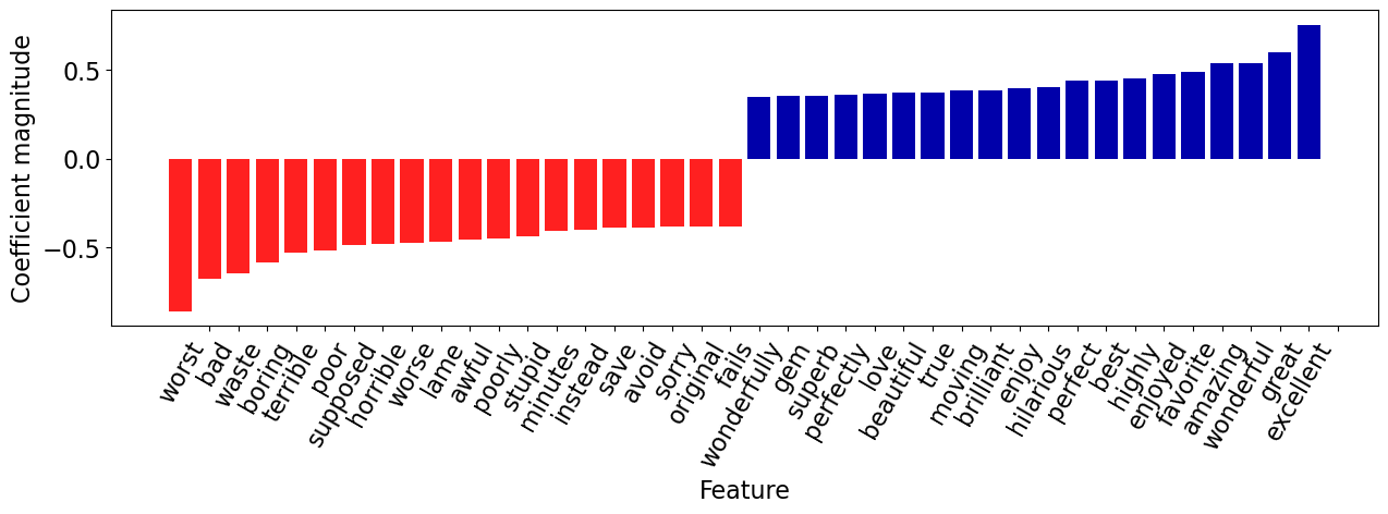
The coefficients make sense!
Let’s visualize the top 20 features.
mglearn.tools.visualize_coefficients(coeffs, feature_names, n_top_features=20)
Let’s explore prediction of the following new review.
fake_reviews = ["It got a bit boring at times but the direction was excellent and the acting was flawless. Overall I enjoyed the movie and I highly recommend it!",
 "The plot was shallower than a kiddie pool in a drought, but hey, at least we now know emojis should stick to texting and avoid the big screen."
]
Let’s get prediction probability scores of the fake review.
best_model.predict(fake_reviews)
array(['pos', 'neg'], dtype=object)
# Get prediction probabilities for fake reviews
best_model.predict_proba(fake_reviews)
array([[0.20880123, 0.79119877],
       [0.64462303, 0.35537697]])
best_model.classes_
array(['neg', 'pos'], dtype=object)
We can find which of the vocabulary words are present in this review:
def plot_coeff_example(model, review, coeffs, feature_names, n_top_feats=6):
    print(review)
    feat_vec = model.named_steps["countvectorizer"].transform([review])
    words_in_ex = feat_vec.toarray().ravel().astype(bool)

    ex_df = pd.DataFrame(
        data=coeffs[words_in_ex],
        index=np.array(feature_names)[words_in_ex],
        columns=["Coefficient"],
    )
    mglearn.tools.visualize_coefficients(
    coeffs[words_in_ex], np.array(feature_names)[words_in_ex], n_top_features=n_top_feats
    )
    return ex_df.sort_values(by=["Coefficient"], ascending=False)
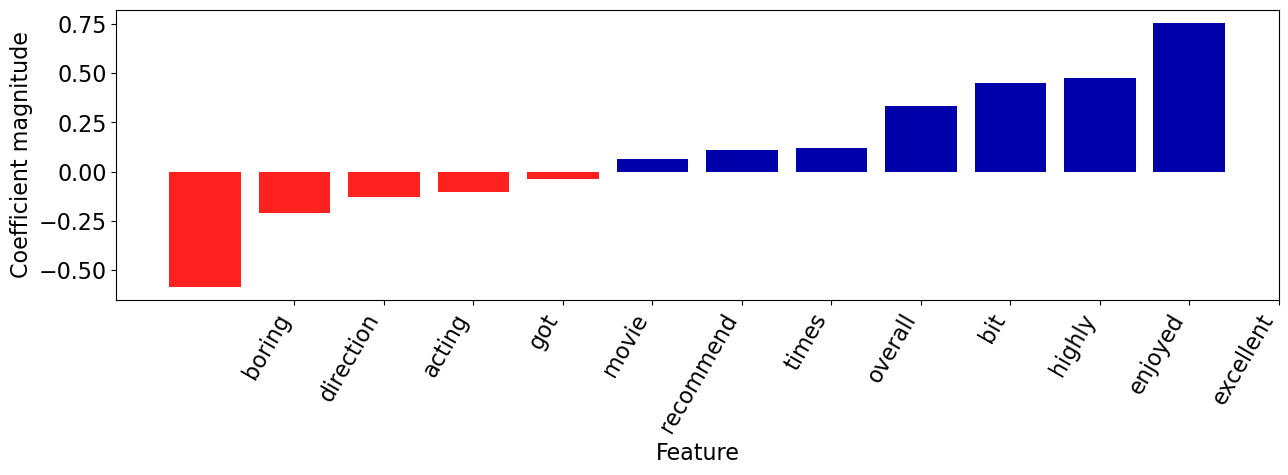
plot_coeff_example(best_model, fake_reviews[0], coeffs, feature_names)
It got a bit boring at times but the direction was excellent and the acting was flawless. Overall I enjoyed the movie and I highly recommend it!
| Coefficient | |
|---|---|
| excellent | 0.754531 |
| enjoyed | 0.475706 |
| highly | 0.450138 |
| bit | 0.332370 |
| overall | 0.119454 |
| times | 0.110395 |
| flawless | 0.078456 |
| recommend | 0.066069 |
| movie | -0.035531 |
| got | -0.104489 |
| acting | -0.128763 |
| direction | -0.207460 |
| boring | -0.582887 |
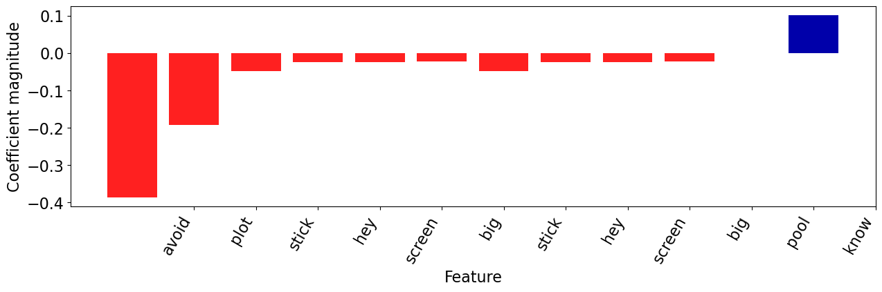
plot_coeff_example(best_model, fake_reviews[1], coeffs, feature_names)
The plot was shallower than a kiddie pool in a drought, but hey, at least we now know emojis should stick to texting and avoid the big screen.
| Coefficient | |
|---|---|
| know | 0.100463 |
| pool | 0.000071 |
| big | -0.021950 |
| screen | -0.024977 |
| hey | -0.025391 |
| stick | -0.047701 |
| plot | -0.192990 |
| avoid | -0.387191 |
Most positive review#
Remember that you can look at the probabilities (confidence) of the classifier’s prediction using the
model.predict_probamethod.Can we find the reviews where our classifier is most certain or least certain?
# only get probabilities associated with pos class
pos_probs = best_model.predict_proba(X_train)[
    :, 1
]  # only get probabilities associated with pos class
pos_probs
array([0.93149138, 0.82269379, 0.8832539 , ..., 0.87023258, 0.08331949,
       0.7576988 ])
What’s the index of the example where the classifier is most certain (highest predict_proba score for positive)?
most_positive_id = np.argmax(pos_probs)
print("True target: %s\n" % (y_train.iloc[most_positive_id]))
print("Predicted target: %s\n" % (best_model.predict(X_train.iloc[[most_positive_id]])[0]))
print("Prediction probability: %0.4f" % (pos_probs[most_positive_id]))
True target: pos

Predicted target: pos

Prediction probability: 1.0000
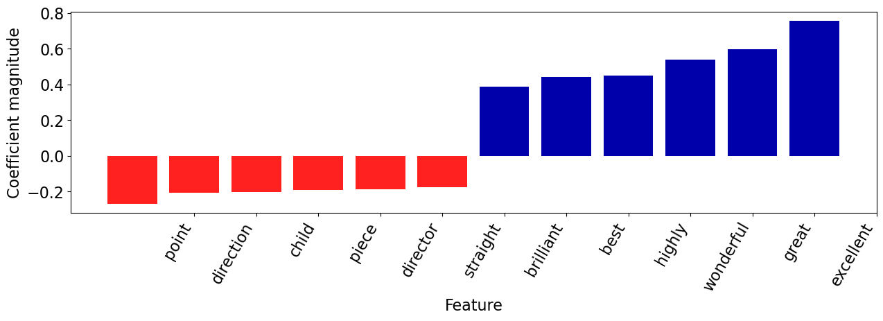
Let’s examine the features associated with the review.
plot_coeff_example(best_model, X_train.iloc[most_positive_id], coeffs, feature_names)
Moving beyond words is this heart breaking story of a divorce which results in a tragic custody battle over a seven year old boy. One of "Kramer v. Kramer's" great strengths is its screenwriter director Robert Benton, who has marvellously adapted Avery Corman's novel to the big screen. He keeps things beautifully simple and most realistic, while delivering all the drama straight from the heart. His talent for telling emotional tales like this was to prove itself again with "Places in the Heart", where he showed, as in "Kramer v. Kramer", that he has a natural ability for working with children. The picture's other strong point is the splendid acting which deservedly received four of the film's nine Academy Award nominations, two of them walking away winners. One of those was Dustin Hoffman (Best Actor), who is superb as frustrated business man Ted Kramer, a man who has forgotten that his wife is a person. As said wife Joanne, Meryl Streep claimed the supporting actress Oscar for a strong, sensitive portrayal of a woman who had lost herself in eight years of marriage. Also nominated was Jane Alexander for her fantastic turn as the Kramer's good friend Margaret. Final word in the acting stakes must go to young Justin Henry, whose incredibly moving performance will find you choking back tears again and again, and a thoroughly deserved Oscar nomination came his way. Brilliant also is Nestor Almendros' cinematography and Jerry Greenberg's timely editing, while musically Henry Purcell's classical piece is used to effect. Truly this is a touching story of how a father and son come to depend on each other when their wife and mother leaves. They grow together, come to know each other and form an entirely new and wonderful relationship. Ted finds himself with new responsibilities and a new outlook on life, and slowly comes to realise why Joanne had to go. Certainly if nothing else, "Kramer v. Kramer" demonstrates that nobody wins when it comes to a custody battle over a young child, especially not the child himself. Saturday, June 10, 1995 - T.V. Strong drama from Avery Corman's novel about the heartache of a custody battle between estranged parents who both feel they have the child's best interests at heart. Aside from a superb screenplay and amazingly controlled direction, both from Robert Benton, it's the superlative cast that make this picture such a winner. Hoffman is brilliant as Ted Kramer, the man torn between his toppling career and the son whom he desperately wants to keep. Excellent too is Streep as the woman lost in eight years of marriage who had to get out before she faded to nothing as a person. In support of these two is a very strong Jane Alexander as mutual friend Margaret, an outstanding Justin Henry as the boy caught in the middle, and a top cast of extras. This highly emotional, heart rending drama more than deserved it's 1979 Academy Awards for best film, best actor (Hoffman) and best supporting actress (Streep). Wednesday, February 28, 1996 - T.V.
| Coefficient | |
|---|---|
| excellent | 0.754531 |
| great | 0.598293 |
| wonderful | 0.539038 |
| highly | 0.450138 |
| best | 0.440914 |
| ... | ... |
| director | -0.189219 |
| piece | -0.192853 |
| child | -0.203941 |
| direction | -0.207460 |
| point | -0.268883 |
187 rows × 1 columns
The review has both positive and negative words but the words with positive coefficients win in this case!
Most negative review#
neg_probs = best_model.predict_proba(X_train)[
    :, 0
]  # only get probabilities associated with neg class
neg_probs
array([0.06850862, 0.17730621, 0.1167461 , ..., 0.12976742, 0.91668051,
       0.2423012 ])
most_negative_id = np.argmax(neg_probs)
print("Review: %s\n" % (X_train.iloc[[most_negative_id]]))
print("True target: %s\n" % (y_train.iloc[most_negative_id]))
print("Predicted target: %s\n" % (best_model.predict(X_train.iloc[[most_negative_id]])[0]))
print("Prediction probability: %0.4f" % (neg_probs[most_negative_id]))
Review: 36555    I made the big mistake of actually watching this whole movie a few nights ago. God I'm still trying to recover. This movie does not even deserve a 1.4 average. IMDb needs to have 0 vote ratings po...
Name: review_pp, dtype: object

True target: neg

Predicted target: neg

Prediction probability: 1.0000
plot_coeff_example(best_model, X_train.iloc[most_negative_id], coeffs, feature_names)
I made the big mistake of actually watching this whole movie a few nights ago. God I'm still trying to recover. This movie does not even deserve a 1.4 average. IMDb needs to have 0 vote ratings possible for movies that really deserve it like this one. A 1.4 is TOO HIGH. I had heard how awful this movie was, but I really did not think a movie could actually be that bad, especially in this day and era. I figured all of the cheesy god awful movies were only from the 1950s and 1960s. My god was I wrong. Trust me folks, this movie REALLY IS THAT BAD. It is beyond horrible; it is beyond pathetic; it is beyond any type of word that I can think of for it. BATTLEFIELD EARTH looks like Best Picture of the Year compared to this movie. SNAKE ISLAND (which up until now was the worst movie I'd ever seen) looks like it deserves a few Oscars compared to this pathetic effort. I seriously can not believe that the makers of this movie thought this was a legitimate serious effort of producing a Hollywood movie. This has no business being called a movie. In the first 25 seconds of the film, I seriously thought I was watching some high school theater class attempting to make a short movie. Or better yet, I thought it was some Saturday night Live ripoff skit of the real thing. I mean, it looks exactly like that. The acting is horrible; the whole movie almost looks like it was shot with a 20 year old VHS video camera. the special effects.......well good lord Bewitched from back in the day had better special effects than this movie. The scene where he gets shot at the door is beyond laughable and beyond cheesy. I mean seriously, my Intro to Acting class from 4 years ago in college, all of us could have put together a better movie than this. And the worst part of the entire movie, where Arthur is naked in the bathroom. Oh my god I almost thew up right there. I have a strong stomach, but wow that was horrible. Some people should never be naked, and he's one of them. The plot of this movie just seems to go absolutely nowhere. They talk about legal issues that we never hear about again; Ben talks about getting into music that we never hear about again; arthur says he is looking for a job and money for college and the next thing we see is he's running a porn shop. Everything about the movie is just horrible. This really doesn't have much to do with my critique, but just so everyone knows, I am not a gay man. I DO however support gay rights and believe we should all be treated as equals. And I would support any gay person in my church, unlike the cruel priest in this movie, who by the way seems to cuss every other word. (WHERE IS THE F*(#*ing white out?) hahaha But I didn't want anyone to think I hated this movie just because of it being about two gay guys. It has nothing to do with that: This would have been just as horrible of a movie if it was Ben & Jill instead of Ben & Arthur. I just watched this movie to see if it really was as bad as they say. And yes it was even WORSE than I had read. Let this be a warning to everyone: ONLY watch this movie if you want to just sit back and laugh at how pathetic some movies in the 21st century can still be. If you watch this movie and are actually expecting a good movie or some entertainment, I have no sympathy for you whatsoever. On a final thought: How in the world are there 7 movies ranked BELOW this on IMDb? There is no way there are 7 movies out there that are worse than this!
| Coefficient | |
|---|---|
| best | 0.440914 |
| job | 0.307902 |
| music | 0.302964 |
| especially | 0.289070 |
| strong | 0.262629 |
| ... | ... |
| awful | -0.455976 |
| worse | -0.474938 |
| horrible | -0.481359 |
| bad | -0.674181 |
| worst | -0.862533 |
173 rows × 1 columns
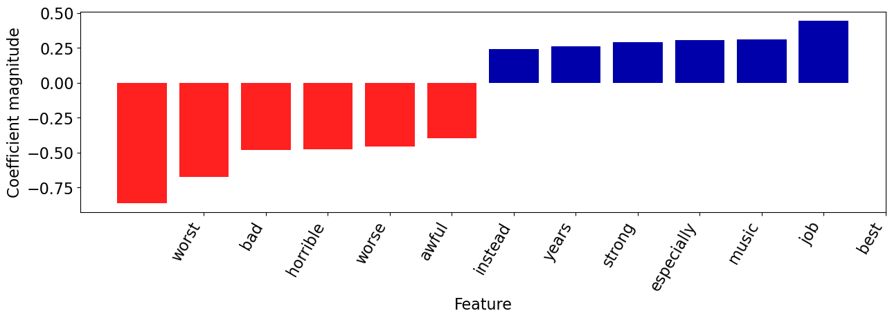
The review has both positive and negative words but the words with negative coefficients win in this case!
❓❓ Questions for you#
Question for you to ponder on#
Is it possible to identify most important features using \(k\)-NNs? What about decision trees?