Lecture 3: Class demo

Image classification using KNNs and SVM RBF

For this demonstration I’m using a subset of Kaggle’s Animal Faces dataset. I’ve put this subset in our course GitHub repository.

The code in this notebook is a bit complicated and you are not expected to understand all the code.

Imports

import sys
import numpy as np
import pandas as pd
import os

sys.path.append(os.path.join(os.path.abspath(".."), "code"))

import matplotlib.pyplot as plt

from sklearn.dummy import DummyClassifier
from plotting_functions import *
from sklearn.model_selection import cross_validate, train_test_split
from utils import *

import torch
from torchvision import datasets, models, transforms, utils
from PIL import Image
from torchvision import transforms
from torchvision.models import vgg16
import matplotlib.pyplot as plt
device = torch.device("cuda:0" if torch.cuda.is_available() else "cpu")

import random
def set_seed(seed=42):
    torch.manual_seed(seed)
    np.random.seed(seed)
    random.seed(seed)
set_seed(seed=42)   

Let’s proceed with reading the data. Since we don’t have tabular data, we are using a slightly more complex method to read it. You don’t need to understand the code provided below.

import glob
IMAGE_SIZE = 200
def read_img_dataset(data_dir):     
    """
    Reads and preprocesses an image dataset from the specified directory.

    Args:
        data_dir (str): The directory path where the dataset is located.

    Returns:
        inputs (Tensor): A batch of preprocessed input images.
        classes (Tensor): The corresponding class labels for the input images.
    """    
    data_transforms = transforms.Compose(
        [
            transforms.Resize((IMAGE_SIZE, IMAGE_SIZE)),     
            transforms.ToTensor(),
            transforms.Normalize([0.5, 0.5, 0.5], [0.5, 0.5, 0.5]),            
        ])
               
    image_dataset = datasets.ImageFolder(root=data_dir, transform=data_transforms)
    dataloader = torch.utils.data.DataLoader(
         image_dataset, batch_size=BATCH_SIZE, shuffle=True, num_workers=0 
    )
    dataset_size = len(image_dataset)
    class_names = image_dataset.classes
    inputs, classes = next(iter(dataloader))
    return inputs, classes

def plot_sample_imgs(inputs):
    plt.figure(figsize=(10, 70)); plt.axis("off"); plt.title("Sample Training Images")
    plt.imshow(np.transpose(utils.make_grid(inputs, padding=1, normalize=True),(1, 2, 0)));

train_dir = "../data/animal_faces/train" # training data
file_names = [image_file for image_file in glob.glob(train_dir + "/*/*.jpg")]
n_images = len(file_names)
BATCH_SIZE = n_images  # because our dataset is quite small
X_anim_train, y_train = read_img_dataset(train_dir)
n_images

---------------------------------------------------------------------------
FileNotFoundError                         Traceback (most recent call last)
Cell In[6], line 5
      3 n_images = len(file_names)
      4 BATCH_SIZE = n_images  # because our dataset is quite small
----> 5 X_anim_train, y_train = read_img_dataset(train_dir)
      6 n_images

Cell In[4], line 21, in read_img_dataset(data_dir)
      4 """
      5 Reads and preprocesses an image dataset from the specified directory.
      6 
   (...)
     12     classes (Tensor): The corresponding class labels for the input images.
     13 """    
     14 data_transforms = transforms.Compose(
     15     [
     16         transforms.Resize((IMAGE_SIZE, IMAGE_SIZE)),     
     17         transforms.ToTensor(),
     18         transforms.Normalize([0.5, 0.5, 0.5], [0.5, 0.5, 0.5]),            
     19     ])
---> 21 image_dataset = datasets.ImageFolder(root=data_dir, transform=data_transforms)
     22 dataloader = torch.utils.data.DataLoader(
     23      image_dataset, batch_size=BATCH_SIZE, shuffle=True, num_workers=0 
     24 )
     25 dataset_size = len(image_dataset)

File ~/miniconda3/envs/cpsc330/lib/python3.10/site-packages/torchvision/datasets/folder.py:309, in ImageFolder.__init__(self, root, transform, target_transform, loader, is_valid_file)
    301 def __init__(
    302     self,
    303     root: str,
   (...)
    307     is_valid_file: Optional[Callable[[str], bool]] = None,
    308 ):
--> 309     super().__init__(
    310         root,
    311         loader,
    312         IMG_EXTENSIONS if is_valid_file is None else None,
    313         transform=transform,
    314         target_transform=target_transform,
    315         is_valid_file=is_valid_file,
    316     )
    317     self.imgs = self.samples

File ~/miniconda3/envs/cpsc330/lib/python3.10/site-packages/torchvision/datasets/folder.py:144, in DatasetFolder.__init__(self, root, loader, extensions, transform, target_transform, is_valid_file)
    134 def __init__(
    135     self,
    136     root: str,
   (...)
    141     is_valid_file: Optional[Callable[[str], bool]] = None,
    142 ) -> None:
    143     super().__init__(root, transform=transform, target_transform=target_transform)
--> 144     classes, class_to_idx = self.find_classes(self.root)
    145     samples = self.make_dataset(self.root, class_to_idx, extensions, is_valid_file)
    147     self.loader = loader

File ~/miniconda3/envs/cpsc330/lib/python3.10/site-packages/torchvision/datasets/folder.py:218, in DatasetFolder.find_classes(self, directory)
    191 def find_classes(self, directory: str) -> Tuple[List[str], Dict[str, int]]:
    192     """Find the class folders in a dataset structured as follows::
    193 
    194         directory/
   (...)
    216         (Tuple[List[str], Dict[str, int]]): List of all classes and dictionary mapping each class to an index.
    217     """
--> 218     return find_classes(directory)

File ~/miniconda3/envs/cpsc330/lib/python3.10/site-packages/torchvision/datasets/folder.py:40, in find_classes(directory)
     35 def find_classes(directory: str) -> Tuple[List[str], Dict[str, int]]:
     36     """Finds the class folders in a dataset.
     37 
     38     See :class:`DatasetFolder` for details.
     39     """
---> 40     classes = sorted(entry.name for entry in os.scandir(directory) if entry.is_dir())
     41     if not classes:
     42         raise FileNotFoundError(f"Couldn't find any class folder in {directory}.")

FileNotFoundError: [Errno 2] No such file or directory: '../data/animal_faces/train'

valid_dir = "../data/animal_faces/valid" # valid data
file_names = [image_file for image_file in glob.glob(valid_dir + "/*/*.jpg")]
n_images = len(file_names)
BATCH_SIZE = n_images  # because our dataset is quite small
X_anim_valid, y_valid = read_img_dataset(valid_dir)
n_images

150

X_train = X_anim_train.numpy()
X_valid = X_anim_valid.numpy()

Let’s examine some of the sample images.

plot_sample_imgs(X_anim_train[0:24,:,:,:])

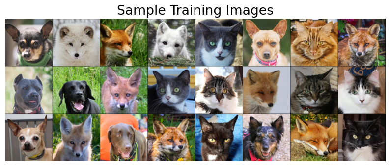
With K-nearest neighbours (KNN), we will attempt to classify an animal face into one of three categories: cat, dog, or wild animal. The idea is that when presented with a new animal face image, we want the model to assign it to one of these three classes based on its similarity to other images within each of these classes.

To train a KNN model, we require tabular data. How can we transform image data, which includes height and width information, into tabular data with meaningful numerical values?

Flattening images and feeding them to K-nearest neighbors (KNN) is one approach. However, in this demonstration, we will explore an alternative method. We will employ a pre-trained image classification model known as ‘desenet’ to obtain a 1024-dimensional meaningful representation of each image. The function provided below accomplishes this task for us. Once again, you are not required to comprehend the code.

def get_features(model, inputs):
    """
    Extracts features from a pre-trained DenseNet model.

    Args:
        model (torch.nn.Module): A pre-trained DenseNet model.
        inputs (torch.Tensor): Input data for feature extraction.

    Returns:
        torch.Tensor: Extracted features from the model.
    """   
    
    with torch.no_grad():  # turn off computational graph stuff
        Z_train = torch.empty((0, 1024))  # Initialize empty tensors
        y_train = torch.empty((0))
        Z_train = torch.cat((Z_train, model(inputs)), dim=0)
    return Z_train.detach().numpy()

densenet = models.densenet121(weights="DenseNet121_Weights.IMAGENET1K_V1")
densenet.classifier = torch.nn.Identity()  # remove that last "classification" layer

X_train.shape

(150, 3, 200, 200)

# Get representations of the train images
Z_train = get_features(
    densenet, X_anim_train, 
)

We now have tabular data.

Z_train.shape

(150, 1024)

pd.DataFrame(Z_train)

	0	1	2	3	4	5	6	7	8	9	...	1014	1015	1016	1017	1018	1019	1020	1021	1022	1023
0	0.000236	0.004594	0.001687	0.002321	0.161429	0.816200	0.000812	0.003663	0.259521	0.000420	...	0.874960	1.427516	1.242740	0.026616	0.210286	0.974181	0.898245	0.904566	0.067099	0.182383
1	0.000128	0.001419	0.002848	0.000313	0.066512	0.442917	0.000423	0.002802	0.056599	0.000839	...	0.805416	0.029395	0.049097	0.319482	0.086078	2.516788	0.864292	3.109580	0.384528	0.046115
2	0.000235	0.006070	0.003593	0.002643	0.098787	0.091632	0.000441	0.003044	0.365898	0.000241	...	0.259085	0.239082	0.084683	1.902342	1.206020	1.027080	0.259025	3.334767	0.428280	0.414404
3	0.000248	0.002965	0.002921	0.000428	0.075668	0.331588	0.000520	0.002987	0.245635	0.000374	...	0.485191	0.157572	0.215166	1.478514	0.014989	0.526783	0.642071	2.119191	1.498163	0.365924
4	0.000296	0.003463	0.001230	0.000890	0.076018	0.726441	0.000685	0.002921	0.194914	0.000281	...	0.449264	0.176026	0.578569	0.152691	0.632296	1.519131	0.781976	0.974530	0.302044	0.614871
...	...	...	...	...	...	...	...	...	...	...	...	...	...	...	...	...	...	...	...	...	...
145	0.000270	0.006250	0.003785	0.002418	0.180926	0.199412	0.000480	0.002477	0.232074	0.000187	...	1.692130	0.727992	0.119121	1.040562	1.431105	0.219714	0.945967	0.758030	0.921435	0.544079
146	0.000316	0.006208	0.003540	0.004469	0.200458	0.398915	0.000475	0.004852	0.196963	0.000329	...	0.620726	1.681427	0.857458	4.337628	0.583973	0.015639	0.373318	0.286325	0.610143	3.533025
147	0.000432	0.001375	0.003088	0.003877	0.154883	0.298043	0.000934	0.001566	0.265483	0.000540	...	0.218867	0.324762	0.039739	3.903423	0.145186	0.221759	1.000562	0.298437	2.578453	0.468994
148	0.000540	0.008286	0.001882	0.001109	0.140371	0.856722	0.000387	0.003272	0.202247	0.000310	...	0.303694	1.546150	2.726269	0.000000	0.495524	0.592507	0.539258	1.308237	0.090579	3.543676
149	0.000163	0.003919	0.003210	0.003910	0.159751	0.295193	0.000460	0.004461	0.401729	0.000328	...	0.916348	0.980963	0.025460	1.526443	1.001512	0.003038	0.068427	3.211725	0.600287	0.032000

150 rows × 1024 columns

# Get representations of the validation images
Z_valid = get_features(
    densenet, X_anim_valid, 
)

Z_valid.shape

(150, 1024)

Dummy model

Let’s examine the baseline accuracy.

from sklearn.dummy import DummyClassifier

dummy = DummyClassifier()
pd.DataFrame(cross_validate(dummy, Z_train, y_train, return_train_score=True))

	fit_time	score_time	test_score	train_score
0	0.000479	0.000418	0.333333	0.333333
1	0.000262	0.000307	0.333333	0.333333
2	0.000239	0.000316	0.333333	0.333333
3	0.000237	0.000294	0.333333	0.333333
4	0.000255	0.000303	0.333333	0.333333

Classification with KNeighborsClassifier

from sklearn.neighbors import KNeighborsClassifier

knn = KNeighborsClassifier()
pd.DataFrame(cross_validate(knn, Z_train, y_train, return_train_score=True))

	fit_time	score_time	test_score	train_score
0	0.000603	0.079621	0.966667	0.991667
1	0.000708	0.009177	1.000000	0.991667
2	0.000501	0.009419	0.933333	0.983333
3	0.000501	0.009090	0.933333	0.991667
4	0.000479	0.008986	0.933333	1.000000

This is with the default n_neighbors. Let’s optimize n_neighbors.

knn.get_params()['n_neighbors']

5

n_neighbors = np.arange(1, 15, 1).tolist()

results_dict = {
    "n_neighbors": [],
    "mean_train_score": [],
    "mean_cv_score": [],
    "std_cv_score": [],
    "std_train_score": [],
}

for k in n_neighbors:
    knn = KNeighborsClassifier(n_neighbors=k)
    scores = cross_validate(knn, Z_train, y_train, return_train_score=True)
    results_dict["n_neighbors"].append(k)

    results_dict["mean_cv_score"].append(np.mean(scores["test_score"]))
    results_dict["mean_train_score"].append(np.mean(scores["train_score"]))
    results_dict["std_cv_score"].append(scores["test_score"].std())
    results_dict["std_train_score"].append(scores["train_score"].std())

results_df = pd.DataFrame(results_dict)
results_df = results_df.set_index("n_neighbors")
results_df

	mean_train_score	mean_cv_score	std_cv_score	std_train_score
n_neighbors
1	1.000000	0.966667	0.021082	0.000000
2	0.988333	0.953333	0.016330	0.006667
3	0.993333	0.953333	0.016330	0.006236
4	0.985000	0.953333	0.016330	0.012247
5	0.991667	0.953333	0.026667	0.005270
6	0.976667	0.940000	0.024944	0.014337
7	0.980000	0.946667	0.016330	0.008498
8	0.968333	0.940000	0.038873	0.020000
9	0.968333	0.926667	0.032660	0.019293
10	0.966667	0.920000	0.033993	0.021082
11	0.963333	0.920000	0.026667	0.017951
12	0.945000	0.913333	0.040000	0.028186
13	0.951667	0.906667	0.032660	0.017795
14	0.945000	0.926667	0.038873	0.022730

results_df[['mean_train_score', 'mean_cv_score']].plot(ylabel='Accuracy', title="k vs. accuracy");

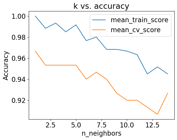
best_k = n_neighbors[np.argmax(results_df['mean_cv_score'])]
best_k

1

Is SVC performing better than k-NN?

C_values = np.logspace(-1, 2, 4)
cv_scores = []
train_scores = []

for C_val in C_values:
    print('C = ', C_val)
    svc = SVC(C=C_val)
    scores = cross_validate(svc, Z_train, y_train, return_train_score=True)
    cv_scores.append(scores['test_score'].mean())
    train_scores.append(scores['train_score'].mean())    

C =  0.1
C =  1.0
C =  10.0
C =  100.0

results_df = pd.DataFrame({"cv": cv_scores, 
                           "train": train_scores},index = C_values)
results_df

	cv	train
0.1	0.973333	0.993333
1.0	1.000000	1.000000
10.0	1.000000	1.000000
100.0	1.000000	1.000000

best_C = C_values[np.argmax(results_df['cv'])]
best_C

1.0

It’s not realistic but we are getting perfect CV accuracy with C=10 and C=100 on our toy dataset. sklearn’s default C =1.0 didn’t give us the best cv score.

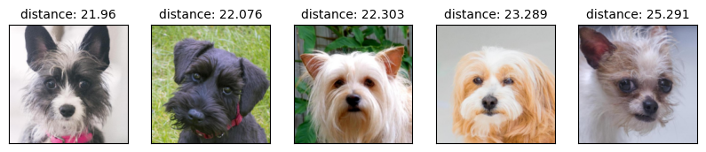
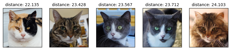
Let’s go back to KNN and manually examine the nearest neighbours.

What are the nearest neighbors?

from sklearn.neighbors import NearestNeighbors
nn = NearestNeighbors()
nn.fit(Z_train)

NearestNeighbors()

In a Jupyter environment, please rerun this cell to show the HTML representation or trust the notebook.
On GitHub, the HTML representation is unable to render, please try loading this page with nbviewer.org.

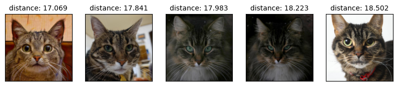
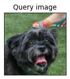
# You do not have to understand this code. 
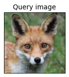
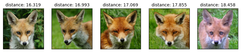
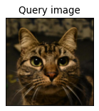
def show_nearest_neighbors(test_idx, nn, Z, X, y):
    distances, neighs = nn.kneighbors([Z[test_idx]])
    neighbors = neighs.ravel()
    plt.figure(figsize=(2,2), dpi=80)
    query_img = X[test_idx].transpose(1, 2, 0)
    query_img = ((X[test_idx].transpose(1, 2, 0) + 1.0) * 0.5 * 255).astype(np.uint8)
    plt.title('Query image', size=12)
    plt.imshow(np.clip(query_img, 0, 255));
    plt.xticks(())
    plt.yticks(())    
    plt.show()
    
    fig, axes = plt.subplots(1, 5, figsize=(10,4), subplot_kw={'xticks':(), 'yticks':()})
    print('Nearest neighbours:')
    
    for ax, dist, img_ind in zip(axes.ravel(), distances.ravel(), neighbors):
        img = X_train[img_ind].transpose(1, 2, 0)
        img = ((X_train[img_ind].transpose(1, 2, 0) + 1.0) * 0.5 * 255).astype(np.uint8)
        ax.imshow(np.clip(img, 0, 255))
        ax.set_title('distance: '+ str(round(dist,3)), size=10 )
    plt.show()

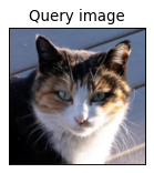
test_idx = [1, 2, 32, 108]
for idx in test_idx: 
    show_nearest_neighbors(idx, nn, Z_valid, X_valid, y_valid)

Nearest neighbours:

Nearest neighbours:

Nearest neighbours:

Nearest neighbours: