
Lectures 5: Class demo#
Imports, Announcements, LOs#
Imports#
# import the libraries
import os
import sys
sys.path.append(os.path.join(os.path.abspath("../"), "code"))
from plotting_functions import *
from utils import *

import matplotlib.pyplot as plt
import numpy as np
import pandas as pd

from sklearn.compose import make_column_transformer
from sklearn.feature_extraction.text import CountVectorizer
from sklearn.preprocessing import StandardScaler, OneHotEncoder

from sklearn.tree import DecisionTreeClassifier
from sklearn.neighbors import KNeighborsClassifier
from sklearn.svm import SVC

%matplotlib inline

pd.set_option("display.max_colwidth", 200)
Incorporating text features in the Spotify dataset#
Recall that we had dropped song_title feature when we worked with the Spotify dataset in Lab 1.
Let’s try to include it in our pipeline and examine whether we get better results.
spotify_df = pd.read_csv("../data/spotify.csv", index_col=0)
X_spotify = spotify_df.drop(columns=["target"])
y_spotify = spotify_df["target"]
---------------------------------------------------------------------------
FileNotFoundError                         Traceback (most recent call last)
Cell In[2], line 1
----> 1 spotify_df = pd.read_csv("../data/spotify.csv", index_col=0)
      2 X_spotify = spotify_df.drop(columns=["target"])
      3 y_spotify = spotify_df["target"]

File ~/miniconda3/envs/571/lib/python3.10/site-packages/pandas/io/parsers/readers.py:948, in read_csv(filepath_or_buffer, sep, delimiter, header, names, index_col, usecols, dtype, engine, converters, true_values, false_values, skipinitialspace, skiprows, skipfooter, nrows, na_values, keep_default_na, na_filter, verbose, skip_blank_lines, parse_dates, infer_datetime_format, keep_date_col, date_parser, date_format, dayfirst, cache_dates, iterator, chunksize, compression, thousands, decimal, lineterminator, quotechar, quoting, doublequote, escapechar, comment, encoding, encoding_errors, dialect, on_bad_lines, delim_whitespace, low_memory, memory_map, float_precision, storage_options, dtype_backend)
    935 kwds_defaults = _refine_defaults_read(
    936     dialect,
    937     delimiter,
   (...)
    944     dtype_backend=dtype_backend,
    945 )
    946 kwds.update(kwds_defaults)
--> 948 return _read(filepath_or_buffer, kwds)

File ~/miniconda3/envs/571/lib/python3.10/site-packages/pandas/io/parsers/readers.py:611, in _read(filepath_or_buffer, kwds)
    608 _validate_names(kwds.get("names", None))
    610 # Create the parser.
--> 611 parser = TextFileReader(filepath_or_buffer, **kwds)
    613 if chunksize or iterator:
    614     return parser

File ~/miniconda3/envs/571/lib/python3.10/site-packages/pandas/io/parsers/readers.py:1448, in TextFileReader.__init__(self, f, engine, **kwds)
   1445     self.options["has_index_names"] = kwds["has_index_names"]
   1447 self.handles: IOHandles | None = None
-> 1448 self._engine = self._make_engine(f, self.engine)

File ~/miniconda3/envs/571/lib/python3.10/site-packages/pandas/io/parsers/readers.py:1705, in TextFileReader._make_engine(self, f, engine)
   1703     if "b" not in mode:
   1704         mode += "b"
-> 1705 self.handles = get_handle(
   1706     f,
   1707     mode,
   1708     encoding=self.options.get("encoding", None),
   1709     compression=self.options.get("compression", None),
   1710     memory_map=self.options.get("memory_map", False),
   1711     is_text=is_text,
   1712     errors=self.options.get("encoding_errors", "strict"),
   1713     storage_options=self.options.get("storage_options", None),
   1714 )
   1715 assert self.handles is not None
   1716 f = self.handles.handle

File ~/miniconda3/envs/571/lib/python3.10/site-packages/pandas/io/common.py:863, in get_handle(path_or_buf, mode, encoding, compression, memory_map, is_text, errors, storage_options)
    858 elif isinstance(handle, str):
    859     # Check whether the filename is to be opened in binary mode.
    860     # Binary mode does not support 'encoding' and 'newline'.
    861     if ioargs.encoding and "b" not in ioargs.mode:
    862         # Encoding
--> 863         handle = open(
    864             handle,
    865             ioargs.mode,
    866             encoding=ioargs.encoding,
    867             errors=errors,
    868             newline="",
    869         )
    870     else:
    871         # Binary mode
    872         handle = open(handle, ioargs.mode)

FileNotFoundError: [Errno 2] No such file or directory: '../data/spotify.csv'
X_train, X_test, y_train, y_test = train_test_split(
    X_spotify, y_spotify, test_size=0.2, random_state=123
)
X_train.shape
(1613, 15)
X_train
| acousticness | danceability | duration_ms | energy | instrumentalness | key | liveness | loudness | mode | speechiness | tempo | time_signature | valence | song_title | artist | |
|---|---|---|---|---|---|---|---|---|---|---|---|---|---|---|---|
| 1505 | 0.004770 | 0.585 | 214740 | 0.614 | 0.000155 | 10 | 0.0762 | -5.594 | 0 | 0.0370 | 114.059 | 4.0 | 0.2730 | Cool for the Summer | Demi Lovato |
| 813 | 0.114000 | 0.665 | 216728 | 0.513 | 0.303000 | 0 | 0.1220 | -7.314 | 1 | 0.3310 | 100.344 | 3.0 | 0.0373 | Damn Son Where'd You Find This? (feat. Kelly Holiday) - Markus Maximus Remix | Markus Maximus |
| 615 | 0.030200 | 0.798 | 216585 | 0.481 | 0.000000 | 7 | 0.1280 | -10.488 | 1 | 0.3140 | 127.136 | 4.0 | 0.6400 | Trill Hoe | Western Tink |
| 319 | 0.106000 | 0.912 | 194040 | 0.317 | 0.000208 | 6 | 0.0723 | -12.719 | 0 | 0.0378 | 99.346 | 4.0 | 0.9490 | Who Is He (And What Is He to You?) | Bill Withers |
| 320 | 0.021100 | 0.697 | 236456 | 0.905 | 0.893000 | 6 | 0.1190 | -7.787 | 0 | 0.0339 | 119.977 | 4.0 | 0.3110 | Acamar | Frankey |
| ... | ... | ... | ... | ... | ... | ... | ... | ... | ... | ... | ... | ... | ... | ... | ... |
| 2012 | 0.001060 | 0.584 | 274404 | 0.932 | 0.002690 | 1 | 0.1290 | -3.501 | 1 | 0.3330 | 74.976 | 4.0 | 0.2110 | Like A Bitch - Kill The Noise Remix | Kill The Noise |
| 1346 | 0.000021 | 0.535 | 203500 | 0.974 | 0.000149 | 10 | 0.2630 | -3.566 | 0 | 0.1720 | 116.956 | 4.0 | 0.4310 | Flag of the Beast | Emmure |
| 1406 | 0.503000 | 0.410 | 256333 | 0.648 | 0.000000 | 7 | 0.2190 | -4.469 | 1 | 0.0362 | 60.391 | 4.0 | 0.3420 | Don't You Cry For Me | Cobi |
| 1389 | 0.705000 | 0.894 | 222307 | 0.161 | 0.003300 | 4 | 0.3120 | -14.311 | 1 | 0.0880 | 104.968 | 4.0 | 0.8180 | 장가갈 수 있을까 Can I Get Married? | Coffeeboy |
| 1534 | 0.623000 | 0.470 | 394920 | 0.156 | 0.187000 | 2 | 0.1040 | -17.036 | 1 | 0.0399 | 118.176 | 4.0 | 0.0591 | Blue Ballad | Phil Woods |
1613 rows × 15 columns
X_train.columns
Index(['acousticness', 'danceability', 'duration_ms', 'energy',
       'instrumentalness', 'key', 'liveness', 'loudness', 'mode',
       'speechiness', 'tempo', 'time_signature', 'valence', 'song_title',
       'artist'],
      dtype='object')
Dummy model#
from sklearn.dummy import DummyClassifier

results = {}
dummy_model = DummyClassifier()
# mean_std_cross_val_scores is defined in ../code/utils.py
results['dummy'] = mean_std_cross_val_scores(dummy_model, X_train, y_train, return_train_score = True)
pd.DataFrame(results)
| dummy | |
|---|---|
| fit_time | 0.000 (+/- 0.000) |
| score_time | 0.000 (+/- 0.000) |
| test_score | 0.508 (+/- 0.001) |
| train_score | 0.508 (+/- 0.000) |
Feature categorization#
X_train.columns
Index(['acousticness', 'danceability', 'duration_ms', 'energy',
       'instrumentalness', 'key', 'liveness', 'loudness', 'mode',
       'speechiness', 'tempo', 'time_signature', 'valence', 'song_title',
       'artist'],
      dtype='object')
X_train["key"].value_counts()
key
1     200
7     169
0     166
9     152
2     145
11    143
5     141
6     127
10    122
8     110
4      88
3      50
Name: count, dtype: int64
X_train["time_signature"].value_counts()
time_signature
4.0    1514
3.0      76
5.0      22
1.0       1
Name: count, dtype: int64
X_train["mode"].value_counts()
mode
1    1002
0     611
Name: count, dtype: int64
Let’s look at the distribution of values in the song_title column.
X_train["song_title"].value_counts()
song_title
Pyramids                                     2
Look At Wrist                                2
Baby                                         2
The One                                      2
Best Friend                                  2
                                            ..
City Of Dreams - Radio Edit                  1
Face It                                      1
The Winner Is - from Little Miss Sunshine    1
History                                      1
Blue Ballad                                  1
Name: count, Length: 1579, dtype: int64
Most of the song titles are unique, which makes sense.
What would happen if we apply one-hot encoding to this feature?
How about encoding this as a text feature?
X_train["artist"].value_counts()
artist
Drake              14
Disclosure         12
Rick Ross          11
WALK THE MOON      10
Crystal Castles     8
                   ..
Classixx            1
Jordan Feliz        1
Travis Hayes        1
The Silvertones     1
Phil Woods          1
Name: count, Length: 1131, dtype: int64
numeric_feats = ['acousticness', 'danceability', 'energy',
                 'instrumentalness', 'liveness', 'loudness',
                 'speechiness', 'tempo', 'valence']
categorical_feats = ['time_signature', 'key']
passthrough_feats = ['mode']
artist_cat_feat = ['artist']
text_feat = 'song_title' # Define the text feature
Important
Note that unlike other feature types we are defining text_feature as a string and not as a list.
Column transformer without song_title and artist features#
preprocessor_no_text = make_column_transformer(
    (StandardScaler(), numeric_feats),
    ("passthrough", passthrough_feats),
    (OneHotEncoder(handle_unknown = "ignore"), categorical_feats),
)
Visualizing the transformed data#
transformed_no_text = preprocessor_no_text.fit_transform(X_train)
transformed_no_text.shape
(1613, 26)
preprocessor_no_text
ColumnTransformer(transformers=[('standardscaler', StandardScaler(),
                                 ['acousticness', 'danceability', 'energy',
                                  'instrumentalness', 'liveness', 'loudness',
                                  'speechiness', 'tempo', 'valence']),
                                ('passthrough', 'passthrough', ['mode']),
                                ('onehotencoder',
                                 OneHotEncoder(handle_unknown='ignore'),
                                 ['time_signature', 'key'])])
In a Jupyter environment, please rerun this cell to show the HTML representation or trust the notebook. On GitHub, the HTML representation is unable to render, please try loading this page with nbviewer.org.
ColumnTransformer(transformers=[('standardscaler', StandardScaler(),
                                 ['acousticness', 'danceability', 'energy',
                                  'instrumentalness', 'liveness', 'loudness',
                                  'speechiness', 'tempo', 'valence']),
                                ('passthrough', 'passthrough', ['mode']),
                                ('onehotencoder',
                                 OneHotEncoder(handle_unknown='ignore'),
['time_signature', 'key'])])['acousticness', 'danceability', 'energy', 'instrumentalness', 'liveness', 'loudness', 'speechiness', 'tempo', 'valence']
StandardScaler()
['mode']
passthrough
['time_signature', 'key']
OneHotEncoder(handle_unknown='ignore')
ohe_feat_names = preprocessor_no_text.named_transformers_["onehotencoder"].get_feature_names_out().tolist()
ohe_feat_names
['time_signature_1.0',
 'time_signature_3.0',
 'time_signature_4.0',
 'time_signature_5.0',
 'key_0',
 'key_1',
 'key_2',
 'key_3',
 'key_4',
 'key_5',
 'key_6',
 'key_7',
 'key_8',
 'key_9',
 'key_10',
 'key_11']
feat_names = numeric_feats + passthrough_feats + ohe_feat_names
pd.DataFrame(transformed_no_text, columns=feat_names)
| acousticness | danceability | energy | instrumentalness | liveness | loudness | speechiness | tempo | valence | mode | ... | key_2 | key_3 | key_4 | key_5 | key_6 | key_7 | key_8 | key_9 | key_10 | key_11 | |
|---|---|---|---|---|---|---|---|---|---|---|---|---|---|---|---|---|---|---|---|---|---|
| 0 | -0.697633 | -0.194548 | -0.318116 | -0.492359 | -0.737898 | 0.395794 | -0.617752 | -0.293827 | -0.908149 | 0.0 | ... | 0.0 | 0.0 | 0.0 | 0.0 | 0.0 | 0.0 | 0.0 | 0.0 | 1.0 | 0.0 |
| 1 | -0.276291 | 0.295726 | -0.795552 | 0.598355 | -0.438792 | -0.052394 | 2.728394 | -0.802595 | -1.861238 | 1.0 | ... | 0.0 | 0.0 | 0.0 | 0.0 | 0.0 | 0.0 | 0.0 | 0.0 | 0.0 | 0.0 |
| 2 | -0.599540 | 1.110806 | -0.946819 | -0.492917 | -0.399607 | -0.879457 | 2.534909 | 0.191274 | 0.575870 | 1.0 | ... | 0.0 | 0.0 | 0.0 | 0.0 | 0.0 | 1.0 | 0.0 | 0.0 | 0.0 | 0.0 |
| 3 | -0.307150 | 1.809445 | -1.722063 | -0.492168 | -0.763368 | -1.460798 | -0.608647 | -0.839616 | 1.825358 | 0.0 | ... | 0.0 | 0.0 | 0.0 | 0.0 | 1.0 | 0.0 | 0.0 | 0.0 | 0.0 | 0.0 |
| 4 | -0.634642 | 0.491835 | 1.057468 | 2.723273 | -0.458384 | -0.175645 | -0.653035 | -0.074294 | -0.754491 | 0.0 | ... | 0.0 | 0.0 | 0.0 | 0.0 | 1.0 | 0.0 | 0.0 | 0.0 | 0.0 | 0.0 |
| ... | ... | ... | ... | ... | ... | ... | ... | ... | ... | ... | ... | ... | ... | ... | ... | ... | ... | ... | ... | ... | ... |
| 1608 | -0.711944 | -0.200676 | 1.185100 | -0.483229 | -0.393077 | 0.941176 | 2.751157 | -1.743639 | -1.158856 | 1.0 | ... | 0.0 | 0.0 | 0.0 | 0.0 | 0.0 | 0.0 | 0.0 | 0.0 | 0.0 | 0.0 |
| 1609 | -0.715953 | -0.500969 | 1.383637 | -0.492380 | 0.482038 | 0.924239 | 0.918743 | -0.186361 | -0.269253 | 0.0 | ... | 0.0 | 0.0 | 0.0 | 0.0 | 0.0 | 0.0 | 0.0 | 0.0 | 1.0 | 0.0 |
| 1610 | 1.224228 | -1.267021 | -0.157395 | -0.492917 | 0.194687 | 0.688940 | -0.626857 | -2.284681 | -0.629138 | 1.0 | ... | 0.0 | 0.0 | 0.0 | 0.0 | 0.0 | 1.0 | 0.0 | 0.0 | 0.0 | 0.0 |
| 1611 | 2.003419 | 1.699134 | -2.459489 | -0.481032 | 0.802042 | -1.875632 | -0.037298 | -0.631064 | 1.295640 | 1.0 | ... | 0.0 | 0.0 | 1.0 | 0.0 | 0.0 | 0.0 | 0.0 | 0.0 | 0.0 | 0.0 |
| 1612 | 1.687114 | -0.899316 | -2.483125 | 0.180574 | -0.556344 | -2.585697 | -0.584746 | -0.141104 | -1.773086 | 1.0 | ... | 1.0 | 0.0 | 0.0 | 0.0 | 0.0 | 0.0 | 0.0 | 0.0 | 0.0 | 0.0 |
1613 rows × 26 columns
Building models#
models = {
    "Decision Tree": DecisionTreeClassifier(),
    "KNN": KNeighborsClassifier(),
    "SVM": SVC()
}

for (name, model) in models.items():
    pipe_model = make_pipeline(preprocessor_no_text, model)
    results[name + " (no_text)"] = mean_std_cross_val_scores(pipe_model, X_train, y_train, return_train_score=True)
pd.DataFrame(results).T
| fit_time | score_time | test_score | train_score | |
|---|---|---|---|---|
| dummy | 0.000 (+/- 0.000) | 0.000 (+/- 0.000) | 0.508 (+/- 0.001) | 0.508 (+/- 0.000) |
| Decision Tree (no_text) | 0.016 (+/- 0.000) | 0.003 (+/- 0.000) | 0.688 (+/- 0.023) | 1.000 (+/- 0.000) |
| KNN (no_text) | 0.005 (+/- 0.001) | 0.015 (+/- 0.020) | 0.676 (+/- 0.028) | 0.788 (+/- 0.009) |
| SVM (no_text) | 0.054 (+/- 0.004) | 0.021 (+/- 0.001) | 0.737 (+/- 0.017) | 0.806 (+/- 0.011) |
Incorporating “song_title” feature#
Let’s incorporate bag-of-words representation of “song_title” feature in our column transformer.
numeric_feats
['acousticness',
 'danceability',
 'energy',
 'instrumentalness',
 'liveness',
 'loudness',
 'speechiness',
 'tempo',
 'valence']
text_feat
'song_title'
preprocessor = make_column_transformer(
    (StandardScaler(), numeric_feats),
    ("passthrough", passthrough_feats),
    (OneHotEncoder(handle_unknown = "ignore"), categorical_feats),
    (CountVectorizer(stop_words="english"), text_feat)
)
# Transform the data
transformed = preprocessor.fit_transform(X_train)
preprocessor
ColumnTransformer(transformers=[('standardscaler', StandardScaler(),
                                 ['acousticness', 'danceability', 'energy',
                                  'instrumentalness', 'liveness', 'loudness',
                                  'speechiness', 'tempo', 'valence']),
                                ('passthrough', 'passthrough', ['mode']),
                                ('onehotencoder',
                                 OneHotEncoder(handle_unknown='ignore'),
                                 ['time_signature', 'key']),
                                ('countvectorizer',
                                 CountVectorizer(stop_words='english'),
                                 'song_title')])
In a Jupyter environment, please rerun this cell to show the HTML representation or trust the notebook. On GitHub, the HTML representation is unable to render, please try loading this page with nbviewer.org.
ColumnTransformer(transformers=[('standardscaler', StandardScaler(),
                                 ['acousticness', 'danceability', 'energy',
                                  'instrumentalness', 'liveness', 'loudness',
                                  'speechiness', 'tempo', 'valence']),
                                ('passthrough', 'passthrough', ['mode']),
                                ('onehotencoder',
                                 OneHotEncoder(handle_unknown='ignore'),
                                 ['time_signature', 'key']),
                                ('countvectorizer',
                                 CountVectorizer(stop_words='english'),
'song_title')])['acousticness', 'danceability', 'energy', 'instrumentalness', 'liveness', 'loudness', 'speechiness', 'tempo', 'valence']
StandardScaler()
['mode']
passthrough
['time_signature', 'key']
OneHotEncoder(handle_unknown='ignore')
song_title
CountVectorizer(stop_words='english')
# Get the vocabulary
vocab = preprocessor.named_transformers_['countvectorizer'].get_feature_names_out()
column_names = numeric_feats + passthrough_feats + ohe_feat_names + vocab.tolist()
len(column_names)
1910
df = pd.DataFrame(transformed.toarray(), columns=column_names)
df
| acousticness | danceability | energy | instrumentalness | liveness | loudness | speechiness | tempo | valence | mode | ... | 너와의 | 루시아 | 변명 | 여기 | 이곳에서 | 이대로 | 있어줘요 | 있을까 | 장가갈 | 지금 | |
|---|---|---|---|---|---|---|---|---|---|---|---|---|---|---|---|---|---|---|---|---|---|
| 0 | -0.697633 | -0.194548 | -0.318116 | -0.492359 | -0.737898 | 0.395794 | -0.617752 | -0.293827 | -0.908149 | 0.0 | ... | 0.0 | 0.0 | 0.0 | 0.0 | 0.0 | 0.0 | 0.0 | 0.0 | 0.0 | 0.0 |
| 1 | -0.276291 | 0.295726 | -0.795552 | 0.598355 | -0.438792 | -0.052394 | 2.728394 | -0.802595 | -1.861238 | 1.0 | ... | 0.0 | 0.0 | 0.0 | 0.0 | 0.0 | 0.0 | 0.0 | 0.0 | 0.0 | 0.0 |
| 2 | -0.599540 | 1.110806 | -0.946819 | -0.492917 | -0.399607 | -0.879457 | 2.534909 | 0.191274 | 0.575870 | 1.0 | ... | 0.0 | 0.0 | 0.0 | 0.0 | 0.0 | 0.0 | 0.0 | 0.0 | 0.0 | 0.0 |
| 3 | -0.307150 | 1.809445 | -1.722063 | -0.492168 | -0.763368 | -1.460798 | -0.608647 | -0.839616 | 1.825358 | 0.0 | ... | 0.0 | 0.0 | 0.0 | 0.0 | 0.0 | 0.0 | 0.0 | 0.0 | 0.0 | 0.0 |
| 4 | -0.634642 | 0.491835 | 1.057468 | 2.723273 | -0.458384 | -0.175645 | -0.653035 | -0.074294 | -0.754491 | 0.0 | ... | 0.0 | 0.0 | 0.0 | 0.0 | 0.0 | 0.0 | 0.0 | 0.0 | 0.0 | 0.0 |
| ... | ... | ... | ... | ... | ... | ... | ... | ... | ... | ... | ... | ... | ... | ... | ... | ... | ... | ... | ... | ... | ... |
| 1608 | -0.711944 | -0.200676 | 1.185100 | -0.483229 | -0.393077 | 0.941176 | 2.751157 | -1.743639 | -1.158856 | 1.0 | ... | 0.0 | 0.0 | 0.0 | 0.0 | 0.0 | 0.0 | 0.0 | 0.0 | 0.0 | 0.0 |
| 1609 | -0.715953 | -0.500969 | 1.383637 | -0.492380 | 0.482038 | 0.924239 | 0.918743 | -0.186361 | -0.269253 | 0.0 | ... | 0.0 | 0.0 | 0.0 | 0.0 | 0.0 | 0.0 | 0.0 | 0.0 | 0.0 | 0.0 |
| 1610 | 1.224228 | -1.267021 | -0.157395 | -0.492917 | 0.194687 | 0.688940 | -0.626857 | -2.284681 | -0.629138 | 1.0 | ... | 0.0 | 0.0 | 0.0 | 0.0 | 0.0 | 0.0 | 0.0 | 0.0 | 0.0 | 0.0 |
| 1611 | 2.003419 | 1.699134 | -2.459489 | -0.481032 | 0.802042 | -1.875632 | -0.037298 | -0.631064 | 1.295640 | 1.0 | ... | 0.0 | 0.0 | 0.0 | 0.0 | 0.0 | 0.0 | 0.0 | 1.0 | 1.0 | 0.0 |
| 1612 | 1.687114 | -0.899316 | -2.483125 | 0.180574 | -0.556344 | -2.585697 | -0.584746 | -0.141104 | -1.773086 | 1.0 | ... | 0.0 | 0.0 | 0.0 | 0.0 | 0.0 | 0.0 | 0.0 | 0.0 | 0.0 | 0.0 |
1613 rows × 1910 columns
Visualizing the vocabulary#
vocab[0:10]
array(['000', '10', '100', '10cm', '11', '112', '12', '1208', '144', '18'],
      dtype=object)
vocab[500:510]
array(['duele', 'duet', 'duke', 'dustland', 'dutchie', 'dynamite',
       'earth', 'easy', 'eazy', 'echelon'], dtype=object)
vocab[1800:1810]
array(['wide', 'wifey', 'wild', 'wildcard', 'wildfire', 'wiley',
       'willing', 'win', 'wind', 'window'], dtype=object)
vocab[0::100]
array(['000', 'ap', 'blind', 'cha', 'dallask', 'duele', 'flashlight',
       'grace', 'icarus', 'lafa', 'making', 'neck', 'pharaohs', 'redeem',
       'seeb', 'soundtrack', 'talons', 'unanswered', 'wide'], dtype=object)
Let’s find songs containing the word earth in them.
earth_index_vocab = np.where(vocab == "earth")[0][0]
earth_index_vocab
506
earth_index_in_df = len(numeric_feats) + len(passthrough_feats) + len(ohe_feat_names) + earth_index_vocab
earth_index_in_df
532
earth_songs = df[df.iloc[:, earth_index_in_df] == 1]
earth_songs.iloc[:, earth_index_in_df - 2 : earth_index_in_df + 2]
| dutchie | dynamite | earth | easy | |
|---|---|---|---|---|
| 380 | 0.0 | 0.0 | 1.0 | 0.0 |
| 639 | 0.0 | 0.0 | 1.0 | 0.0 |
earth_songs.index
Index([380, 639], dtype='int64')
X_train.iloc[earth_songs.index]["song_title"]
1851             Softest Place On Earth
1948    Earth Song - Remastered Version
Name: song_title, dtype: object
Model building#
models = {
    "Decision Tree": DecisionTreeClassifier(),
    "KNN": KNeighborsClassifier(),
    "SVM": SVC()
}

for (name, model) in models.items():
    pipe_model = make_pipeline(preprocessor, model)
    results[name + " (text)"] = mean_std_cross_val_scores(pipe_model, X_train, y_train, return_train_score=True)
pd.DataFrame(results).T
| fit_time | score_time | test_score | train_score | |
|---|---|---|---|---|
| dummy | 0.000 (+/- 0.000) | 0.000 (+/- 0.000) | 0.508 (+/- 0.001) | 0.508 (+/- 0.000) |
| Decision Tree (no_text) | 0.016 (+/- 0.000) | 0.003 (+/- 0.000) | 0.688 (+/- 0.023) | 1.000 (+/- 0.000) |
| KNN (no_text) | 0.005 (+/- 0.001) | 0.015 (+/- 0.020) | 0.676 (+/- 0.028) | 0.788 (+/- 0.009) |
| SVM (no_text) | 0.054 (+/- 0.004) | 0.021 (+/- 0.001) | 0.737 (+/- 0.017) | 0.806 (+/- 0.011) |
| Decision Tree (text) | 0.035 (+/- 0.002) | 0.005 (+/- 0.001) | 0.700 (+/- 0.027) | 1.000 (+/- 0.000) |
| KNN (text) | 0.012 (+/- 0.002) | 0.031 (+/- 0.004) | 0.682 (+/- 0.028) | 0.786 (+/- 0.010) |
| SVM (text) | 0.059 (+/- 0.003) | 0.014 (+/- 0.001) | 0.733 (+/- 0.027) | 0.866 (+/- 0.004) |
Not a big difference in the results.
Seems like there is more overfitting when we included the
song_titlefeature.The training score of SVC is much higher when we include all features. Hyperparameter optimization of
Candgammamay help.
What about the
artistcolumn?Does it make sense to apply BOW encoding to it?
Let’s look at the distribution of values in the
artistcolumn.
X_train['artist'].value_counts()
artist
Drake              14
Disclosure         12
Rick Ross          11
WALK THE MOON      10
Crystal Castles     8
                   ..
Classixx            1
Jordan Feliz        1
Travis Hayes        1
The Silvertones     1
Phil Woods          1
Name: count, Length: 1131, dtype: int64
most_frequent = X_train["artist"].value_counts().iloc[:15]
most_frequent
artist
Drake              14
Disclosure         12
Rick Ross          11
WALK THE MOON      10
Crystal Castles     8
Big Time Rush       8
FIDLAR              8
Fall Out Boy        8
Demi Lovato         7
Kanye West          7
Kina Grannis        7
Backstreet Boys     7
Beach House         6
Young Thug          6
*NSYNC              6
Name: count, dtype: int64
preprocessor_artist = make_column_transformer(
    (StandardScaler(), numeric_feats),
    ("passthrough", passthrough_feats),
    (OneHotEncoder(handle_unknown = "ignore"), categorical_feats),
    (OneHotEncoder(dtype=int, handle_unknown="ignore", categories=[most_frequent.index.values]), artist_cat_feat),
    (CountVectorizer(max_features = 100, stop_words="english"), text_feat)
)
models = {
    "Decision Tree": DecisionTreeClassifier(),
    "KNN": KNeighborsClassifier(),
    "SVM": SVC()
}

for (name, model) in models.items():
    pipe_model = make_pipeline(preprocessor_artist, model)
    results[name + " (all)"] = mean_std_cross_val_scores(pipe_model, X_train, y_train, return_train_score=True)
pd.DataFrame(results).T
| fit_time | score_time | test_score | train_score | |
|---|---|---|---|---|
| dummy | 0.000 (+/- 0.000) | 0.000 (+/- 0.000) | 0.508 (+/- 0.001) | 0.508 (+/- 0.000) |
| Decision Tree (no_text) | 0.016 (+/- 0.000) | 0.003 (+/- 0.000) | 0.688 (+/- 0.023) | 1.000 (+/- 0.000) |
| KNN (no_text) | 0.005 (+/- 0.001) | 0.015 (+/- 0.020) | 0.676 (+/- 0.028) | 0.788 (+/- 0.009) |
| SVM (no_text) | 0.054 (+/- 0.004) | 0.021 (+/- 0.001) | 0.737 (+/- 0.017) | 0.806 (+/- 0.011) |
| Decision Tree (text) | 0.035 (+/- 0.002) | 0.005 (+/- 0.001) | 0.700 (+/- 0.027) | 1.000 (+/- 0.000) |
| KNN (text) | 0.012 (+/- 0.002) | 0.031 (+/- 0.004) | 0.682 (+/- 0.028) | 0.786 (+/- 0.010) |
| SVM (text) | 0.059 (+/- 0.003) | 0.014 (+/- 0.001) | 0.733 (+/- 0.027) | 0.866 (+/- 0.004) |
| Decision Tree (all) | 0.028 (+/- 0.001) | 0.005 (+/- 0.001) | 0.684 (+/- 0.035) | 1.000 (+/- 0.000) |
| KNN (all) | 0.012 (+/- 0.000) | 0.026 (+/- 0.001) | 0.681 (+/- 0.032) | 0.792 (+/- 0.008) |
| SVM (all) | 0.052 (+/- 0.004) | 0.013 (+/- 0.000) | 0.741 (+/- 0.027) | 0.833 (+/- 0.006) |
Tiny bit improvement in the mean CV scores but we are still overfitting.
(Optional) Incorporating text features in the restaurant survey dataset#
Do you recall the restaurants survey you completed at the start of the course?
Let’s use that data for this demo. You’ll find a wrangled version in the course repository.
df = pd.read_csv('../data/cleaned_restaurant_data.csv')
df
| north_america | eat_out_freq | age | n_people | price | food_type | noise_level | good_server | comments | restaurant_name | target | |
|---|---|---|---|---|---|---|---|---|---|---|---|
| 0 | Yes | 3.0 | 29 | 10.0 | 120.0 | Italian | medium | Yes | Ambience | NaN | dislike |
| 1 | Yes | 2.0 | 23 | 3.0 | 20.0 | Canadian/American | no music | No | food tastes bad | NaN | dislike |
| 2 | Yes | 2.0 | 21 | 20.0 | 15.0 | Chinese | medium | Yes | bad food | NaN | dislike |
| 3 | No | 2.0 | 24 | 14.0 | 18.0 | Other | medium | No | Overall vibe on the restaurant | NaN | dislike |
| 4 | Yes | 5.0 | 23 | 30.0 | 20.0 | Chinese | medium | Yes | A bad day | NaN | dislike |
| ... | ... | ... | ... | ... | ... | ... | ... | ... | ... | ... | ... |
| 959 | No | 10.0 | 22 | NaN | NaN | NaN | NaN | NaN | NaN | NaN | like |
| 960 | Yes | 1.0 | 20 | NaN | NaN | NaN | NaN | NaN | NaN | NaN | like |
| 961 | No | 1.0 | 22 | 40.0 | 50.0 | Chinese | medium | Yes | The self service sauce table is very clean and the sauces were always filled up. | Haidilao | like |
| 962 | Yes | 3.0 | 21 | NaN | NaN | NaN | NaN | NaN | NaN | NaN | like |
| 963 | Yes | 3.0 | 27 | 20.0 | 22.0 | Other | medium | Yes | Lots of meat that was very soft and tasty. Hearty and amazing broth. Good noodle thickness and consistency | Uno Beef Noodle | like |
964 rows × 11 columns
df.describe()
| eat_out_freq | age | n_people | price | |
|---|---|---|---|---|
| count | 964.000000 | 964.000000 | 6.960000e+02 | 696.000000 |
| mean | 2.585187 | 23.975104 | 1.439254e+04 | 1472.179152 |
| std | 2.246486 | 4.556716 | 3.790481e+05 | 37903.575636 |
| min | 0.000000 | 10.000000 | -2.000000e+00 | 0.000000 |
| 25% | 1.000000 | 21.000000 | 1.000000e+01 | 18.000000 |
| 50% | 2.000000 | 22.000000 | 2.000000e+01 | 25.000000 |
| 75% | 3.000000 | 26.000000 | 3.000000e+01 | 40.000000 |
| max | 15.000000 | 46.000000 | 1.000000e+07 | 1000000.000000 |
Are there any unusual values in this data that you notice? Let’s get rid of these outliers.
upperbound_price = 200
lowerbound_people = 1
df = df[~(df['price'] > 200)]
restaurant_df = df[~(df['n_people'] < lowerbound_people)]
restaurant_df.shape
(942, 11)
restaurant_df.describe()
| eat_out_freq | age | n_people | price | |
|---|---|---|---|---|
| count | 942.000000 | 942.000000 | 674.000000 | 674.000000 |
| mean | 2.598057 | 23.992569 | 24.973294 | 34.023279 |
| std | 2.257787 | 4.582570 | 22.016660 | 29.018622 |
| min | 0.000000 | 10.000000 | 1.000000 | 0.000000 |
| 25% | 1.000000 | 21.000000 | 10.000000 | 18.000000 |
| 50% | 2.000000 | 22.000000 | 20.000000 | 25.000000 |
| 75% | 3.000000 | 26.000000 | 30.000000 | 40.000000 |
| max | 15.000000 | 46.000000 | 200.000000 | 200.000000 |
Data splitting#
We aim to predict whether a restaurant is liked or disliked.
# Separate `X` and `y`.

X = restaurant_df.drop(columns=['target'])
y = restaurant_df['target']
Below I’m perturbing this data just to demonstrate a few concepts. Don’t do it in real life.
X.at[459, 'food_type'] = 'Quebecois'
X['price'] = X['price'] * 100
# Split the data

X_train, X_test, y_train, y_test = train_test_split(X, y, test_size=0.2, random_state=123)
EDA#
X_train.hist(bins=20, figsize=(12, 8));
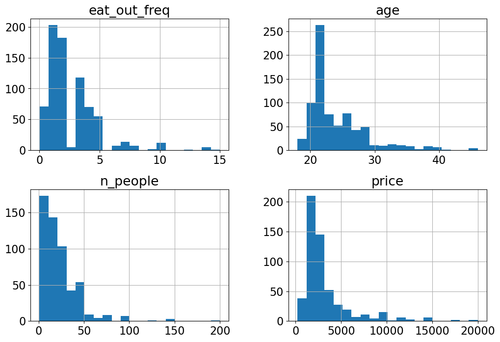
Do you see anything interesting in these plots?
X_train['food_type'].value_counts()
food_type
Other                189
Canadian/American    131
Chinese              102
Indian                36
Italian               32
Thai                  20
Fusion                18
Mexican               17
fusion                 3
Quebecois              1
Name: count, dtype: int64
Error in data collection? Probably “Fusion” and “fusion” categories should be combined?
X_train['food_type'] = X_train['food_type'].replace("fusion", "Fusion")
X_test['food_type'] = X_test['food_type'].replace("fusion", "Fusion")
X_train['food_type'].value_counts()
food_type
Other                189
Canadian/American    131
Chinese              102
Indian                36
Italian               32
Fusion                21
Thai                  20
Mexican               17
Quebecois              1
Name: count, dtype: int64
Again, usually we should spend lots of time in EDA, but let’s stop here so that we have time to learn about transformers and pipelines.
Dummy Classifier#
from sklearn.dummy import DummyClassifier

results_df = {}
dummy = DummyClassifier()
results_df['dummy'] = mean_std_cross_val_scores(dummy, X_train, y_train, return_train_score=True)
pd.DataFrame(results_df)
| dummy | |
|---|---|
| fit_time | 0.001 (+/- 0.000) |
| score_time | 0.001 (+/- 0.000) |
| test_score | 0.515 (+/- 0.002) |
| train_score | 0.515 (+/- 0.000) |
We have a relatively balanced distribution of both ‘like’ and ‘dislike’ classes.
Preprocessing#
How can we horizontally stack
preprocessed numeric features,
preprocessed binary features,
preprocessed ordinal features, and
preprocessed categorical features?
Let’s define a column transformer.
numeric_feats = ['age', 'n_people', 'price'] # Continuous and quantitative features
categorical_feats = ['north_america', 'food_type'] # Discrete and qualitative features
binary_feats = ['good_server'] # Categorical features with only two possible values
ordinal_feats = ['noise_level'] # Some natural ordering in the categories
noise_cats = ['no music', 'low', 'medium', 'high', 'crazy loud']
drop_feats = ['comments', 'restaurant_name', 'eat_out_freq'] # Dropping text feats and `eat_out_freq` because it's not that useful
X_train['noise_level'].value_counts()
noise_level
medium        232
low           186
high           75
no music       37
crazy loud     18
Name: count, dtype: int64
noise_levels = ["no music", "low", "medium", "high", "crazy loud"]
from sklearn.impute import SimpleImputer
from sklearn.preprocessing import StandardScaler
from sklearn.preprocessing import OneHotEncoder
from sklearn.preprocessing import OrdinalEncoder

from sklearn.compose import make_column_transformer

numeric_transformer = make_pipeline(SimpleImputer(strategy="median"),
                                    StandardScaler())
binary_transformer = make_pipeline(SimpleImputer(strategy="most_frequent"),
                                    OneHotEncoder(drop="if_binary"))
ordinal_transformer = make_pipeline(SimpleImputer(strategy="most_frequent"),
                                    OrdinalEncoder(categories=[noise_levels]))
categorical_transformer = make_pipeline(SimpleImputer(strategy="most_frequent"),
                                    OneHotEncoder(sparse_output=False, handle_unknown="ignore"))

preprocessor = make_column_transformer(
    (numeric_transformer, numeric_feats),
    (binary_transformer, binary_feats),
    (ordinal_transformer, ordinal_feats),
    (categorical_transformer, categorical_feats),
    ("drop", drop_feats)
)
How does the transformed data look like?
transformed = preprocessor.fit_transform(X_train)
transformed.shape
(753, 17)
preprocessor
ColumnTransformer(transformers=[('pipeline-1',
                                 Pipeline(steps=[('simpleimputer',
                                                  SimpleImputer(strategy='median')),
                                                 ('standardscaler',
                                                  StandardScaler())]),
                                 ['age', 'n_people', 'price']),
                                ('pipeline-2',
                                 Pipeline(steps=[('simpleimputer',
                                                  SimpleImputer(strategy='most_frequent')),
                                                 ('onehotencoder',
                                                  OneHotEncoder(drop='if_binary'))]),
                                 ['good_server']),
                                ('pipeline-3',...
                                                  OrdinalEncoder(categories=[['no '
                                                                              'music',
                                                                              'low',
                                                                              'medium',
                                                                              'high',
                                                                              'crazy '
                                                                              'loud']]))]),
                                 ['noise_level']),
                                ('pipeline-4',
                                 Pipeline(steps=[('simpleimputer',
                                                  SimpleImputer(strategy='most_frequent')),
                                                 ('onehotencoder',
                                                  OneHotEncoder(handle_unknown='ignore',
                                                                sparse_output=False))]),
                                 ['north_america', 'food_type']),
                                ('drop', 'drop',
                                 ['comments', 'restaurant_name',
                                  'eat_out_freq'])])
In a Jupyter environment, please rerun this cell to show the HTML representation or trust the notebook. On GitHub, the HTML representation is unable to render, please try loading this page with nbviewer.org.
ColumnTransformer(transformers=[('pipeline-1',
                                 Pipeline(steps=[('simpleimputer',
                                                  SimpleImputer(strategy='median')),
                                                 ('standardscaler',
                                                  StandardScaler())]),
                                 ['age', 'n_people', 'price']),
                                ('pipeline-2',
                                 Pipeline(steps=[('simpleimputer',
                                                  SimpleImputer(strategy='most_frequent')),
                                                 ('onehotencoder',
                                                  OneHotEncoder(drop='if_binary'))]),
                                 ['good_server']),
                                ('pipeline-3',...
                                                  OrdinalEncoder(categories=[['no '
                                                                              'music',
                                                                              'low',
                                                                              'medium',
                                                                              'high',
                                                                              'crazy '
                                                                              'loud']]))]),
                                 ['noise_level']),
                                ('pipeline-4',
                                 Pipeline(steps=[('simpleimputer',
                                                  SimpleImputer(strategy='most_frequent')),
                                                 ('onehotencoder',
                                                  OneHotEncoder(handle_unknown='ignore',
                                                                sparse_output=False))]),
                                 ['north_america', 'food_type']),
                                ('drop', 'drop',
                                 ['comments', 'restaurant_name',
'eat_out_freq'])])['age', 'n_people', 'price']
SimpleImputer(strategy='median')
StandardScaler()
['good_server']
SimpleImputer(strategy='most_frequent')
OneHotEncoder(drop='if_binary')
['noise_level']
SimpleImputer(strategy='most_frequent')
OrdinalEncoder(categories=[['no music', 'low', 'medium', 'high', 'crazy loud']])
['north_america', 'food_type']
SimpleImputer(strategy='most_frequent')
OneHotEncoder(handle_unknown='ignore', sparse_output=False)
['comments', 'restaurant_name', 'eat_out_freq']
drop
# Getting feature names from a column transformer
ohe_feat_names = preprocessor.named_transformers_['pipeline-4']['onehotencoder'].get_feature_names_out(categorical_feats).tolist()
ohe_feat_names
["north_america_Don't want to share",
 'north_america_No',
 'north_america_Yes',
 'food_type_Canadian/American',
 'food_type_Chinese',
 'food_type_Fusion',
 'food_type_Indian',
 'food_type_Italian',
 'food_type_Mexican',
 'food_type_Other',
 'food_type_Quebecois',
 'food_type_Thai']
numeric_feats
['age', 'n_people', 'price']
feat_names = numeric_feats + binary_feats + ordinal_feats + ohe_feat_names
transformed
array([[-0.66941678,  0.31029469, -0.36840629, ...,  0.        ,
         0.        ,  0.        ],
       [-0.66941678,  0.31029469, -0.05422496, ...,  0.        ,
         0.        ,  0.        ],
       [-0.89515383,  0.82336432, -0.25058829, ...,  0.        ,
         0.        ,  0.        ],
       ...,
       [-0.89515383, -0.97237936, -0.64331495, ...,  0.        ,
         0.        ,  0.        ],
       [-0.89515383, -0.20277493, -0.25058829, ...,  1.        ,
         0.        ,  0.        ],
       [-0.89515383,  1.33643394, -0.05422496, ...,  0.        ,
         0.        ,  0.        ]])
pd.DataFrame(transformed, columns = feat_names)
| age | n_people | price | good_server | noise_level | north_america_Don't want to share | north_america_No | north_america_Yes | food_type_Canadian/American | food_type_Chinese | food_type_Fusion | food_type_Indian | food_type_Italian | food_type_Mexican | food_type_Other | food_type_Quebecois | food_type_Thai | |
|---|---|---|---|---|---|---|---|---|---|---|---|---|---|---|---|---|---|
| 0 | -0.669417 | 0.310295 | -0.368406 | 0.0 | 3.0 | 0.0 | 1.0 | 0.0 | 0.0 | 1.0 | 0.0 | 0.0 | 0.0 | 0.0 | 0.0 | 0.0 | 0.0 |
| 1 | -0.669417 | 0.310295 | -0.054225 | 1.0 | 1.0 | 0.0 | 0.0 | 1.0 | 1.0 | 0.0 | 0.0 | 0.0 | 0.0 | 0.0 | 0.0 | 0.0 | 0.0 |
| 2 | -0.895154 | 0.823364 | -0.250588 | 1.0 | 2.0 | 0.0 | 1.0 | 0.0 | 1.0 | 0.0 | 0.0 | 0.0 | 0.0 | 0.0 | 0.0 | 0.0 | 0.0 |
| 3 | -0.669417 | -0.202775 | -0.250588 | 1.0 | 2.0 | 0.0 | 0.0 | 1.0 | 0.0 | 0.0 | 0.0 | 0.0 | 0.0 | 0.0 | 0.0 | 1.0 | 0.0 |
| 4 | 0.007794 | -0.202775 | -0.054225 | 1.0 | 3.0 | 0.0 | 0.0 | 1.0 | 0.0 | 0.0 | 0.0 | 1.0 | 0.0 | 0.0 | 0.0 | 0.0 | 0.0 |
| ... | ... | ... | ... | ... | ... | ... | ... | ... | ... | ... | ... | ... | ... | ... | ... | ... | ... |
| 748 | 0.685006 | -0.715845 | -0.643315 | 1.0 | 2.0 | 0.0 | 1.0 | 0.0 | 0.0 | 1.0 | 0.0 | 0.0 | 0.0 | 0.0 | 0.0 | 0.0 | 0.0 |
| 749 | 0.007794 | -0.613231 | -0.918224 | 1.0 | 2.0 | 0.0 | 1.0 | 0.0 | 0.0 | 0.0 | 0.0 | 0.0 | 0.0 | 0.0 | 1.0 | 0.0 | 0.0 |
| 750 | -0.895154 | -0.972379 | -0.643315 | 0.0 | 1.0 | 0.0 | 0.0 | 1.0 | 1.0 | 0.0 | 0.0 | 0.0 | 0.0 | 0.0 | 0.0 | 0.0 | 0.0 |
| 751 | -0.895154 | -0.202775 | -0.250588 | 1.0 | 2.0 | 0.0 | 0.0 | 1.0 | 0.0 | 0.0 | 0.0 | 0.0 | 0.0 | 0.0 | 1.0 | 0.0 | 0.0 |
| 752 | -0.895154 | 1.336434 | -0.054225 | 1.0 | 3.0 | 1.0 | 0.0 | 0.0 | 0.0 | 1.0 | 0.0 | 0.0 | 0.0 | 0.0 | 0.0 | 0.0 | 0.0 |
753 rows × 17 columns
We have new columns for the categorical features. Let’s create a pipeline with the preprocessor and SVC.
from sklearn.tree import DecisionTreeClassifier
from sklearn.neighbors import KNeighborsClassifier
from sklearn.svm import SVC
models = {
    "Decision Tree": DecisionTreeClassifier(),
    "KNN": KNeighborsClassifier(),
    "SVM": SVC()
}

for (name, model) in models.items():
    pipe_num_model = make_pipeline(SimpleImputer(strategy="median"), StandardScaler(), model)
    results_df[name +' (numeric-only)'] = mean_std_cross_val_scores(pipe_num_model, X_train[numeric_feats], y_train, return_train_score=True)
pd.DataFrame(results_df).T
| fit_time | score_time | test_score | train_score | |
|---|---|---|---|---|
| dummy | 0.001 (+/- 0.000) | 0.001 (+/- 0.000) | 0.515 (+/- 0.002) | 0.515 (+/- 0.000) |
| Decision Tree (numeric-only) | 0.003 (+/- 0.000) | 0.001 (+/- 0.000) | 0.497 (+/- 0.038) | 0.833 (+/- 0.010) |
| KNN (numeric-only) | 0.003 (+/- 0.001) | 0.004 (+/- 0.000) | 0.525 (+/- 0.034) | 0.674 (+/- 0.015) |
| SVM (numeric-only) | 0.012 (+/- 0.000) | 0.005 (+/- 0.000) | 0.587 (+/- 0.033) | 0.623 (+/- 0.006) |
for (name, model) in models.items():
    pipe_model = make_pipeline(preprocessor, model)
    results_df[name + '(non-text feats)'] = mean_std_cross_val_scores(pipe_model, X_train, y_train, return_train_score=True)
pd.DataFrame(results_df).T
| fit_time | score_time | test_score | train_score | |
|---|---|---|---|---|
| dummy | 0.001 (+/- 0.000) | 0.001 (+/- 0.000) | 0.515 (+/- 0.002) | 0.515 (+/- 0.000) |
| Decision Tree (numeric-only) | 0.003 (+/- 0.000) | 0.001 (+/- 0.000) | 0.497 (+/- 0.038) | 0.833 (+/- 0.010) |
| KNN (numeric-only) | 0.003 (+/- 0.001) | 0.004 (+/- 0.000) | 0.525 (+/- 0.034) | 0.674 (+/- 0.015) |
| SVM (numeric-only) | 0.012 (+/- 0.000) | 0.005 (+/- 0.000) | 0.587 (+/- 0.033) | 0.623 (+/- 0.006) |
| Decision Tree(non-text feats) | 0.009 (+/- 0.000) | 0.003 (+/- 0.000) | 0.590 (+/- 0.039) | 0.889 (+/- 0.008) |
| KNN(non-text feats) | 0.008 (+/- 0.000) | 0.004 (+/- 0.000) | 0.598 (+/- 0.023) | 0.737 (+/- 0.008) |
| SVM(non-text feats) | 0.019 (+/- 0.000) | 0.008 (+/- 0.000) | 0.687 (+/- 0.011) | 0.733 (+/- 0.008) |
We are getting better results when we include numeric, categorical, binary, ordinal features.
Incorporating text features#
We haven’t incorporated the comments feature into our pipeline yet, even though it holds significant value in indicating whether the restaurant was liked or not.
X_train
| north_america | eat_out_freq | age | n_people | price | food_type | noise_level | good_server | comments | restaurant_name | |
|---|---|---|---|---|---|---|---|---|---|---|
| 80 | No | 2.0 | 21 | 30.0 | 2200.0 | Chinese | high | No | The environment was very not clean. The food tasted awful. | NaN |
| 934 | Yes | 4.0 | 21 | 30.0 | 3000.0 | Canadian/American | low | Yes | The building and the room gave a very comfy feeling. Immediately after sitting down it felt like we were right at home. | NaN |
| 911 | No | 4.0 | 20 | 40.0 | 2500.0 | Canadian/American | medium | Yes | I was hungry | Chambar |
| 459 | Yes | 5.0 | 21 | NaN | NaN | Quebecois | NaN | NaN | NaN | NaN |
| 62 | Yes | 2.0 | 24 | 20.0 | 3000.0 | Indian | high | Yes | bad taste | east is east |
| ... | ... | ... | ... | ... | ... | ... | ... | ... | ... | ... |
| 106 | No | 3.0 | 27 | 10.0 | 1500.0 | Chinese | medium | Yes | Food wasn't great. | NaN |
| 333 | No | 1.0 | 24 | 12.0 | 800.0 | Other | medium | Yes | NaN | NaN |
| 393 | Yes | 4.0 | 20 | 5.0 | 1500.0 | Canadian/American | low | No | NaN | NaN |
| 376 | Yes | 5.0 | 20 | NaN | NaN | NaN | NaN | NaN | NaN | NaN |
| 525 | Don't want to share | 4.0 | 20 | 50.0 | 3000.0 | Chinese | high | Yes | NaN | Haidilao |
753 rows × 10 columns
Let’s create bag-of-words representation of the comments feature. But first we need to impute the rows where there are no comments. There is a small complication if we want to put SimpleImputer and CountVectorizer in a pipeline.
SimpleImputertakes a 2D array as input and produced 2D array as output.CountVectorizertakes a 1D array as input.
To deal with this, we will use sklearn’s FunctionTransformer to convert the 2D output of SimpleImputer into a 1D array which can be passed to CountVectorizer as input.
from sklearn.preprocessing import FunctionTransformer
from sklearn.feature_extraction.text import CountVectorizer

reshape_for_countvectorizer = FunctionTransformer(lambda X: X.squeeze(), validate=False)
text_transformer = make_pipeline(SimpleImputer(strategy="constant", fill_value="missing"),
                          reshape_for_countvectorizer,
                          CountVectorizer(stop_words="english"))
text_pipe = make_pipeline(text_transformer, SVC())
cross_val_score(text_pipe, X_train[['comments']], y_train).mean()
0.6493951434878588
Pretty good scores just with text features! Let’s examine the transformed data.
transformed = text_transformer.fit_transform(X_train[['comments']], y_train)
transformed
<753x548 sparse matrix of type '<class 'numpy.int64'>'
	with 1841 stored elements in Compressed Sparse Row format>
It’s a sparse matrix. Let’s explore the the vocabulary.
vocab = text_transformer.named_steps["countvectorizer"].get_feature_names_out()
vocab[:10]
array(['18', '30', '40mins', '65', 'actually', 'addition', 'affordable',
       'alcohol', 'ale', 'allergic'], dtype=object)
vocab[0:10]
array(['18', '30', '40mins', '65', 'actually', 'addition', 'affordable',
       'alcohol', 'ale', 'allergic'], dtype=object)
vocab[200:210]
array(['fusion', 'games', 'gave', 'general', 'genuinely', 'getting',
       'ginger', 'girlfriends', 'gluten', 'going'], dtype=object)
vocab[500:600]
array(['undressed', 'unfresh', 'uni', 'unique', 'unreasonable', 'upset',
       'usual', 'uwu', 'value', 'vancouver', 'variety', 'vds', 've',
       'vegan', 'vibe', 'vibes', 'vietnamese', 'view', 'visit', 'wait',
       'waited', 'waiter', 'waiters', 'waiting', 'waitress', 'walking',
       'want', 'warm', 'washrooms', 'wasn', 'water', 'watery', 'way',
       'weekend', 'went', 'wet', 'wife', 'wind', 'window', 'wine',
       'wings', 'winter', 'work', 'worst', 'wrong', 'yelling', 'yield',
       'yummy'], dtype=object)
vocab[0::20]
array(['18', 'ask', 'better', 'cash', 'closing', 'country', 'dessert',
       'drunk', 'expecting', 'figuring', 'fusion', 'having', 'impeccable',
       'knowledgeable', 'love', 'nice', 'pain', 'played', 'quality',
       'removed', 'sauces', 'sitting', 'spoke', 'tacky', 'time',
       'undressed', 'waited', 'wings'], dtype=object)
Do we get better scores if we combine all features? Let’s define a column transformer which carries out
imputation and scaling on numeric features
imputation and one-hot encoding with
drop="if_binary"on binary featuresimputation and one-hot encoding with
handle_unknown="ignore"on categorical featuresimputation, reshaping, and bag-of-words transformation on the text feature
from sklearn.feature_extraction.text import CountVectorizer
text_feat = ['comments']

preprocessor_all = make_column_transformer(
    (numeric_transformer, numeric_feats),
    (binary_transformer, binary_feats),
    (ordinal_transformer, ordinal_feats),
    (categorical_transformer, categorical_feats),
    (text_transformer, text_feat),
    ("drop", drop_feats)
)
preprocessor_all.fit_transform(X_train)
<753x565 sparse matrix of type '<class 'numpy.float64'>'
	with 6927 stored elements in Compressed Sparse Row format>
for (name, model) in models.items():
    pipe_model = make_pipeline(text_transformer, model)
    results_df[name + '(text)'] = mean_std_cross_val_scores(pipe_model, X_train[['comments']], y_train, return_train_score=True)
pd.DataFrame(results_df).T
| fit_time | score_time | test_score | train_score | |
|---|---|---|---|---|
| dummy | 0.001 (+/- 0.000) | 0.001 (+/- 0.000) | 0.515 (+/- 0.002) | 0.515 (+/- 0.000) |
| Decision Tree (numeric-only) | 0.003 (+/- 0.000) | 0.001 (+/- 0.000) | 0.497 (+/- 0.038) | 0.833 (+/- 0.010) |
| KNN (numeric-only) | 0.003 (+/- 0.001) | 0.004 (+/- 0.000) | 0.525 (+/- 0.034) | 0.674 (+/- 0.015) |
| SVM (numeric-only) | 0.012 (+/- 0.000) | 0.005 (+/- 0.000) | 0.587 (+/- 0.033) | 0.623 (+/- 0.006) |
| Decision Tree(non-text feats) | 0.009 (+/- 0.000) | 0.003 (+/- 0.000) | 0.590 (+/- 0.039) | 0.889 (+/- 0.008) |
| KNN(non-text feats) | 0.008 (+/- 0.000) | 0.004 (+/- 0.000) | 0.598 (+/- 0.023) | 0.737 (+/- 0.008) |
| SVM(non-text feats) | 0.019 (+/- 0.000) | 0.008 (+/- 0.000) | 0.687 (+/- 0.011) | 0.733 (+/- 0.008) |
| Decision Tree(text) | 0.008 (+/- 0.001) | 0.001 (+/- 0.000) | 0.618 (+/- 0.036) | 0.735 (+/- 0.004) |
| KNN(text) | 0.004 (+/- 0.000) | 0.006 (+/- 0.002) | 0.572 (+/- 0.023) | 0.646 (+/- 0.026) |
| SVM(text) | 0.010 (+/- 0.000) | 0.003 (+/- 0.000) | 0.649 (+/- 0.022) | 0.728 (+/- 0.005) |
for (name, model) in models.items():
    pipe_model = make_pipeline(preprocessor_all, model)
    results_df[name + '(all)'] = mean_std_cross_val_scores(pipe_model, X_train, y_train, return_train_score=True)
pd.DataFrame(results_df).T
| fit_time | score_time | test_score | train_score | |
|---|---|---|---|---|
| dummy | 0.001 (+/- 0.000) | 0.001 (+/- 0.000) | 0.515 (+/- 0.002) | 0.515 (+/- 0.000) |
| Decision Tree (numeric-only) | 0.003 (+/- 0.000) | 0.001 (+/- 0.000) | 0.497 (+/- 0.038) | 0.833 (+/- 0.010) |
| KNN (numeric-only) | 0.003 (+/- 0.001) | 0.004 (+/- 0.000) | 0.525 (+/- 0.034) | 0.674 (+/- 0.015) |
| SVM (numeric-only) | 0.012 (+/- 0.000) | 0.005 (+/- 0.000) | 0.587 (+/- 0.033) | 0.623 (+/- 0.006) |
| Decision Tree(non-text feats) | 0.009 (+/- 0.000) | 0.003 (+/- 0.000) | 0.590 (+/- 0.039) | 0.889 (+/- 0.008) |
| KNN(non-text feats) | 0.008 (+/- 0.000) | 0.004 (+/- 0.000) | 0.598 (+/- 0.023) | 0.737 (+/- 0.008) |
| SVM(non-text feats) | 0.019 (+/- 0.000) | 0.008 (+/- 0.000) | 0.687 (+/- 0.011) | 0.733 (+/- 0.008) |
| Decision Tree(text) | 0.008 (+/- 0.001) | 0.001 (+/- 0.000) | 0.618 (+/- 0.036) | 0.735 (+/- 0.004) |
| KNN(text) | 0.004 (+/- 0.000) | 0.006 (+/- 0.002) | 0.572 (+/- 0.023) | 0.646 (+/- 0.026) |
| SVM(text) | 0.010 (+/- 0.000) | 0.003 (+/- 0.000) | 0.649 (+/- 0.022) | 0.728 (+/- 0.005) |
| Decision Tree(all) | 0.016 (+/- 0.001) | 0.005 (+/- 0.001) | 0.624 (+/- 0.022) | 0.893 (+/- 0.006) |
| KNN(all) | 0.013 (+/- 0.000) | 0.012 (+/- 0.001) | 0.625 (+/- 0.027) | 0.748 (+/- 0.015) |
| SVM(all) | 0.023 (+/- 0.000) | 0.008 (+/- 0.001) | 0.699 (+/- 0.017) | 0.786 (+/- 0.008) |
Some improvement when we combine all features!