Lecture 03: PCA applications class demo

import os
import random
import sys

import numpy as np
import pandas as pd

sys.path.append(os.path.join(os.path.abspath(".."), "code"))

import matplotlib.pyplot as plt
import seaborn as sns
from plotting_functions import *
from sklearn.decomposition import PCA
from sklearn.pipeline import make_pipeline
from sklearn.preprocessing import StandardScaler

plt.rcParams["font.size"] = 10
plt.rcParams["figure.figsize"] = (5, 4)
%matplotlib inline
pd.set_option("display.max_colwidth", 0)

%config InlineBackend.figure_formats = ['svg']

DATA_DIR = os.path.join(os.path.abspath(".."), "data/")

---------------------------------------------------------------------------
ImportError                               Traceback (most recent call last)
Cell In[1], line 12
     10 import matplotlib.pyplot as plt
     11 import seaborn as sns
---> 12 from plotting_functions import *
     13 from sklearn.decomposition import PCA
     14 from sklearn.pipeline import make_pipeline

File ~/MDS/2024-25/563/DSCI_563_unsup-learn/lectures/code/plotting_functions.py:7
      5 import matplotlib.pyplot as plt
      6 from matplotlib.colors import ListedColormap, colorConverter, LinearSegmentedColormap
----> 7 from scipy.spatial import distance
      8 from sklearn.metrics import euclidean_distances
      9 from sklearn.manifold import MDS

File ~/miniforge3/envs/jbook/lib/python3.12/site-packages/scipy/spatial/__init__.py:110
      1 """
      2 =============================================================
      3 Spatial algorithms and data structures (:mod:`scipy.spatial`)
   (...)
    107    QhullError
    108 """  # noqa: E501
--> 110 from ._kdtree import *
    111 from ._ckdtree import *  # type: ignore[import-not-found]
    112 from ._qhull import *

File ~/miniforge3/envs/jbook/lib/python3.12/site-packages/scipy/spatial/_kdtree.py:4
      1 # Copyright Anne M. Archibald 2008
      2 # Released under the scipy license
      3 import numpy as np
----> 4 from ._ckdtree import cKDTree, cKDTreeNode  # type: ignore[import-not-found]
      6 __all__ = ['minkowski_distance_p', 'minkowski_distance',
      7            'distance_matrix',
      8            'Rectangle', 'KDTree']
     11 def minkowski_distance_p(x, y, p=2):

File _ckdtree.pyx:11, in init scipy.spatial._ckdtree()

File ~/miniforge3/envs/jbook/lib/python3.12/site-packages/scipy/sparse/__init__.py:315
    312 from ._sputils import get_index_dtype, safely_cast_index_arrays
    314 # For backward compatibility with v0.19.
--> 315 from . import csgraph
    317 # Deprecated namespaces, to be removed in v2.0.0
    318 from . import (
    319     base, bsr, compressed, construct, coo, csc, csr, data, dia, dok, extract,
    320     lil, sparsetools, sputils
    321 )

File ~/miniforge3/envs/jbook/lib/python3.12/site-packages/scipy/sparse/csgraph/__init__.py:187
    158 __docformat__ = "restructuredtext en"
    160 __all__ = ['connected_components',
    161            'laplacian',
    162            'shortest_path',
   (...)
    184            'csgraph_to_masked',
    185            'NegativeCycleError']
--> 187 from ._laplacian import laplacian
    188 from ._shortest_path import (
    189     shortest_path, floyd_warshall, dijkstra, bellman_ford, johnson, yen,
    190     NegativeCycleError
    191 )
    192 from ._traversal import (
    193     breadth_first_order, depth_first_order, breadth_first_tree,
    194     depth_first_tree, connected_components
    195 )

File ~/miniforge3/envs/jbook/lib/python3.12/site-packages/scipy/sparse/csgraph/_laplacian.py:7
      5 import numpy as np
      6 from scipy.sparse import issparse
----> 7 from scipy.sparse.linalg import LinearOperator
      8 from scipy.sparse._sputils import convert_pydata_sparse_to_scipy, is_pydata_spmatrix
     11 ###############################################################################
     12 # Graph laplacian

File ~/miniforge3/envs/jbook/lib/python3.12/site-packages/scipy/sparse/linalg/__init__.py:129
      1 """
      2 Sparse linear algebra (:mod:`scipy.sparse.linalg`)
      3 ==================================================
   (...)
    126 
    127 """
--> 129 from ._isolve import *
    130 from ._dsolve import *
    131 from ._interface import *

File ~/miniforge3/envs/jbook/lib/python3.12/site-packages/scipy/sparse/linalg/_isolve/__init__.py:4
      1 "Iterative Solvers for Sparse Linear Systems"
      3 #from info import __doc__
----> 4 from .iterative import *
      5 from .minres import minres
      6 from .lgmres import lgmres

File ~/miniforge3/envs/jbook/lib/python3.12/site-packages/scipy/sparse/linalg/_isolve/iterative.py:5
      3 from scipy.sparse.linalg._interface import LinearOperator
      4 from .utils import make_system
----> 5 from scipy.linalg import get_lapack_funcs
      7 __all__ = ['bicg', 'bicgstab', 'cg', 'cgs', 'gmres', 'qmr']
     10 def _get_atol_rtol(name, b_norm, atol=0., rtol=1e-5):

File ~/miniforge3/envs/jbook/lib/python3.12/site-packages/scipy/linalg/__init__.py:203
      1 """
      2 ====================================
      3 Linear algebra (:mod:`scipy.linalg`)
   (...)
    200 
    201 """  # noqa: E501
--> 203 from ._misc import *
    204 from ._cythonized_array_utils import *
    205 from ._basic import *

File ~/miniforge3/envs/jbook/lib/python3.12/site-packages/scipy/linalg/_misc.py:3
      1 import numpy as np
      2 from numpy.linalg import LinAlgError
----> 3 from .blas import get_blas_funcs
      4 from .lapack import get_lapack_funcs
      6 __all__ = ['LinAlgError', 'LinAlgWarning', 'norm']

File ~/miniforge3/envs/jbook/lib/python3.12/site-packages/scipy/linalg/blas.py:213
    210 import numpy as np
    211 import functools
--> 213 from scipy.linalg import _fblas
    214 try:
    215     from scipy.linalg import _cblas

ImportError: dlopen(/Users/kvarada/miniforge3/envs/jbook/lib/python3.12/site-packages/scipy/linalg/_fblas.cpython-312-darwin.so, 0x0002): Library not loaded: @rpath/libgfortran.5.dylib
  Referenced from: <0B9C315B-A1DD-3527-88DB-4B90531D343F> /Users/kvarada/miniforge3/envs/jbook/lib/libopenblas.0.dylib
  Reason: tried: '/Users/kvarada/miniforge3/envs/jbook/lib/libgfortran.5.dylib' (duplicate LC_RPATH '@loader_path'), '/Users/kvarada/miniforge3/envs/jbook/lib/libgfortran.5.dylib' (duplicate LC_RPATH '@loader_path'), '/Users/kvarada/miniforge3/envs/jbook/lib/python3.12/site-packages/scipy/linalg/../../../../libgfortran.5.dylib' (duplicate LC_RPATH '@loader_path'), '/Users/kvarada/miniforge3/envs/jbook/lib/python3.12/site-packages/scipy/linalg/../../../../libgfortran.5.dylib' (duplicate LC_RPATH '@loader_path'), '/Users/kvarada/miniforge3/envs/jbook/bin/../lib/libgfortran.5.dylib' (duplicate LC_RPATH '@loader_path'), '/Users/kvarada/miniforge3/envs/jbook/bin/../lib/libgfortran.5.dylib' (duplicate LC_RPATH '@loader_path'), '/usr/local/lib/libgfortran.5.dylib' (no such file), '/usr/lib/libgfortran.5.dylib' (no such file, not in dyld cache)

PCA applications

There are tons of applications of PCA. In this section we’ll look at a few example applications.

Big five personality traits

Have you heard of the Big Five personality traits:

• Extroversion: Reflects sociability, energy, and enthusiasm

• Openness: Measures creativity, curiosity, and willingness to try new experiences.

• Agreeableness: Represents compassion, kindness, and cooperativeness.

• Conscientiousness: Reflects discipline, organization, and reliability.

• Neuroticism: Measures emotional stability and tendency toward negative emotions.

These were identified using PCA based on a large-scale personality data set obtained from the Open-Source Psychometrics Project: https://openpsychometrics.org/.

This dataset contains several thousand responses to an online personality survey consisting of 50 statements rated on a 5-point likert scale.

You can see the statements themselves at this link.

## Big 5 data
bf = pd.read_csv("https://remiller1450.github.io/data/big5data.csv", sep='\t')

## Split the personality questions from the demographics
bf_demo = bf[['race','age','engnat','gender','hand','source','country']]
bf_demo

	race	age	engnat	gender	hand	source	country
0	3	53	1	1	1	1	US
1	13	46	1	2	1	1	US
2	1	14	2	2	1	1	PK
3	3	19	2	2	1	1	RO
4	11	25	2	2	1	2	US
...	...	...	...	...	...	...	...
19714	11	15	1	2	1	2	SG
19715	3	37	1	2	1	2	US
19716	5	16	2	1	1	2	US
19717	12	16	1	1	1	5	NG
19718	3	35	1	1	1	1	US

19719 rows × 7 columns

The rest of the columns are the responses to an online personality survey consisting of 50 statements rated on a 5-point likert scale, where

• 0=missed

• 1=Disagree

• 3=Neutral

• 5=Agree

Let’s examine these columns:

bf_qs = bf.drop(columns=['race','age','engnat','gender','hand','source','country'])
bf_qs

	E1	E2	E3	E4	E5	E6	E7	E8	E9	E10	...	O1	O2	O3	O4	O5	O6	O7	O8	O9	O10
0	4	2	5	2	5	1	4	3	5	1	...	4	1	3	1	5	1	4	2	5	5
1	2	2	3	3	3	3	1	5	1	5	...	3	3	3	3	2	3	3	1	3	2
2	5	1	1	4	5	1	1	5	5	1	...	4	5	5	1	5	1	5	5	5	5
3	2	5	2	4	3	4	3	4	4	5	...	4	3	5	2	4	2	5	2	5	5
4	3	1	3	3	3	1	3	1	3	5	...	3	1	1	1	3	1	3	1	5	3
...	...	...	...	...	...	...	...	...	...	...	...	...	...	...	...	...	...	...	...	...	...
19714	1	4	3	5	4	3	1	2	1	5	...	1	3	5	3	4	1	4	2	5	3
19715	2	3	2	3	2	3	2	4	4	4	...	1	2	3	2	3	3	4	2	3	3
19716	2	5	4	5	5	5	1	2	1	5	...	5	3	1	3	4	1	1	5	5	5
19717	1	4	2	3	2	4	1	3	4	5	...	3	2	5	3	4	1	5	3	5	5
19718	2	3	1	5	3	3	3	2	2	4	...	5	1	5	1	4	1	5	5	5	5

19719 rows × 50 columns

Let’s store the mapping of column names and actual questions from this link in a dictionary.

# Dictionary mapping feature names to actual questions
questions_dict = {
    "E1": "I am the life of the party.",
    "E2": "I don't talk a lot.",
    "E3": "I feel comfortable around people.",
    "E4": "I keep in the background.",
    "E5": "I start conversations.",
    "E6": "I have little to say.",
    "E7": "I talk to a lot of different people at parties.",
    "E8": "I don't like to draw attention to myself.",
    "E9": "I don't mind being the center of attention.",
    "E10": "I am quiet around strangers.",
    "N1": "I get stressed out easily.",
    "N2": "I am relaxed most of the time.",
    "N3": "I worry about things.",
    "N4": "I seldom feel blue.",
    "N5": "I am easily disturbed.",
    "N6": "I get upset easily.",
    "N7": "I change my mood a lot.",
    "N8": "I have frequent mood swings.",
    "N9": "I get irritated easily.",
    "N10": "I often feel blue.",
    "A1": "I feel little concern for others.",
    "A2": "I am interested in people.",
    "A3": "I insult people.",
    "A4": "I sympathize with others' feelings.",
    "A5": "I am not interested in other people's problems.",
    "A6": "I have a soft heart.",
    "A7": "I am not really interested in others.",
    "A8": "I take time out for others.",
    "A9": "I feel others' emotions.",
    "A10": "I make people feel at ease.",
    "C1": "I am always prepared.",
    "C2": "I leave my belongings around.",
    "C3": "I pay attention to details.",
    "C4": "I make a mess of things.",
    "C5": "I get chores done right away.",
    "C6": "I often forget to put things back in their proper place.",
    "C7": "I like order.",
    "C8": "I shirk my duties.",
    "C9": "I follow a schedule.",
    "C10": "I am exacting in my work.",
    "O1": "I have a rich vocabulary.",
    "O2": "I have difficulty understanding abstract ideas.",
    "O3": "I have a vivid imagination.",
    "O4": "I am not interested in abstract ideas.",
    "O5": "I have excellent ideas.",
    "O6": "I do not have a good imagination.",
    "O7": "I am quick to understand things.",
    "O8": "I use difficult words.",
    "O9": "I spend time reflecting on things.",
    "O10": "I am full of ideas."
}

bf_qs.shape

(19719, 50)

❓❓ Questions for you

• Why would applying PCA be useful in this scenario?

from sklearn.decomposition import PCA
pca_bfq = PCA(n_components=5, random_state=42)
pca_bfq.fit(bf_qs)

PCA(n_components=5, random_state=42)

In a Jupyter environment, please rerun this cell to show the HTML representation or trust the notebook.
On GitHub, the HTML representation is unable to render, please try loading this page with nbviewer.org.

pca_bfq.explained_variance_ratio_.sum()

np.float64(0.4645454150547113)

The first 5 components are coverting 46% of the information. Good to know!

# Get the components
W = pca_bfq.components_

# Get the feature names
feature_names = bf_qs.columns

# Create a DataFrame for better visualization
components_df = pd.DataFrame(W.T, columns=[f'PC{i}' for i in range(W.shape[0])], index=feature_names)

# Display the most influential features for each component
for i in range(W.shape[0]):
    print(f"\nTop positive features for PC{i}:\n")
    top_pos_features = components_df.iloc[:, i].sort_values(ascending=False).head(10)
    for feature, value in top_pos_features.items():
        print(f"{feature}: {questions_dict.get(feature, 'Unknown question')} (Score: {value:.4f})")

    print(f"\nTop negative features for PC{i}:\n")
    top_neg_features = components_df.iloc[:, i].sort_values(ascending=True).head(10)
    for feature, value in top_neg_features.items():
        print(f"{feature}: {questions_dict.get(feature, 'Unknown question')} (Score: {value:.4f})")

    print("\n" + "-"*50 + "\n")

Top positive features for PC0:

E7: I talk to a lot of different people at parties. (Score: 0.2635)
E3: I feel comfortable around people. (Score: 0.2526)
E5: I start conversations. (Score: 0.2409)
E9: I don't mind being the center of attention. (Score: 0.1923)
E1: I am the life of the party. (Score: 0.1869)
A10: I make people feel at ease. (Score: 0.1469)
A2: I am interested in people. (Score: 0.1409)
N2: I am relaxed most of the time. (Score: 0.1288)
C5: I get chores done right away. (Score: 0.1080)
N4: I seldom feel blue. (Score: 0.1079)

Top negative features for PC0:

E10: I am quiet around strangers. (Score: -0.2235)
N10: I often feel blue. (Score: -0.2222)
E4: I keep in the background. (Score: -0.2116)
N8: I have frequent mood swings. (Score: -0.2052)
N9: I get irritated easily. (Score: -0.1973)
E6: I have little to say. (Score: -0.1967)
E2: I don't talk a lot. (Score: -0.1956)
N6: I get upset easily. (Score: -0.1944)
N7: I change my mood a lot. (Score: -0.1854)
N1: I get stressed out easily. (Score: -0.1793)

--------------------------------------------------


Top positive features for PC1:

N8: I have frequent mood swings. (Score: 0.2663)
N7: I change my mood a lot. (Score: 0.2525)
N6: I get upset easily. (Score: 0.2462)
E7: I talk to a lot of different people at parties. (Score: 0.2176)
C6: I often forget to put things back in their proper place. (Score: 0.2085)
N1: I get stressed out easily. (Score: 0.2071)
N9: I get irritated easily. (Score: 0.2044)
C4: I make a mess of things. (Score: 0.2034)
E9: I don't mind being the center of attention. (Score: 0.1984)
C2: I leave my belongings around. (Score: 0.1973)

Top negative features for PC1:

E2: I don't talk a lot. (Score: -0.2271)
E8: I don't like to draw attention to myself. (Score: -0.1674)
E6: I have little to say. (Score: -0.1587)
E4: I keep in the background. (Score: -0.1483)
E10: I am quiet around strangers. (Score: -0.1358)
C5: I get chores done right away. (Score: -0.1231)
A7: I am not really interested in others. (Score: -0.1221)
N2: I am relaxed most of the time. (Score: -0.1111)
C1: I am always prepared. (Score: -0.1111)
A5: I am not interested in other people's problems. (Score: -0.1084)

--------------------------------------------------


Top positive features for PC2:

C9: I follow a schedule. (Score: 0.2718)
C5: I get chores done right away. (Score: 0.2397)
A6: I have a soft heart. (Score: 0.2313)
A4: I sympathize with others' feelings. (Score: 0.2306)
A9: I feel others' emotions. (Score: 0.2273)
C7: I like order. (Score: 0.2237)
N3: I worry about things. (Score: 0.2056)
N1: I get stressed out easily. (Score: 0.1985)
A8: I take time out for others. (Score: 0.1746)
C1: I am always prepared. (Score: 0.1689)

Top negative features for PC2:

C6: I often forget to put things back in their proper place. (Score: -0.2440)
C2: I leave my belongings around. (Score: -0.2286)
A5: I am not interested in other people's problems. (Score: -0.1914)
A3: I insult people. (Score: -0.1884)
A1: I feel little concern for others. (Score: -0.1869)
C8: I shirk my duties. (Score: -0.1696)
C4: I make a mess of things. (Score: -0.1506)
A7: I am not really interested in others. (Score: -0.1479)
N2: I am relaxed most of the time. (Score: -0.1454)
E9: I don't mind being the center of attention. (Score: -0.1270)

--------------------------------------------------


Top positive features for PC3:

O8: I use difficult words. (Score: 0.3518)
O1: I have a rich vocabulary. (Score: 0.3224)
O10: I am full of ideas. (Score: 0.2381)
O3: I have a vivid imagination. (Score: 0.2346)
O9: I spend time reflecting on things. (Score: 0.1939)
O5: I have excellent ideas. (Score: 0.1810)
O7: I am quick to understand things. (Score: 0.1777)
C2: I leave my belongings around. (Score: 0.1683)
C6: I often forget to put things back in their proper place. (Score: 0.1262)
E4: I keep in the background. (Score: 0.1185)

Top negative features for PC3:

O2: I have difficulty understanding abstract ideas. (Score: -0.3167)
O4: I am not interested in abstract ideas. (Score: -0.2953)
O6: I do not have a good imagination. (Score: -0.2328)
A1: I feel little concern for others. (Score: -0.1877)
C5: I get chores done right away. (Score: -0.1422)
E7: I talk to a lot of different people at parties. (Score: -0.1281)
E1: I am the life of the party. (Score: -0.1164)
E3: I feel comfortable around people. (Score: -0.1018)
N5: I am easily disturbed. (Score: -0.1016)
A5: I am not interested in other people's problems. (Score: -0.0977)

--------------------------------------------------


Top positive features for PC4:

O8: I use difficult words. (Score: 0.2359)
A5: I am not interested in other people's problems. (Score: 0.2298)
A1: I feel little concern for others. (Score: 0.2212)
A3: I insult people. (Score: 0.2068)
A7: I am not really interested in others. (Score: 0.1963)
N9: I get irritated easily. (Score: 0.1923)
C1: I am always prepared. (Score: 0.1904)
O1: I have a rich vocabulary. (Score: 0.1874)
C7: I like order. (Score: 0.1863)
C9: I follow a schedule. (Score: 0.1850)

Top negative features for PC4:

A4: I sympathize with others' feelings. (Score: -0.2255)
C6: I often forget to put things back in their proper place. (Score: -0.2194)
A6: I have a soft heart. (Score: -0.2133)
C2: I leave my belongings around. (Score: -0.1963)
A9: I feel others' emotions. (Score: -0.1712)
A8: I take time out for others. (Score: -0.1564)
A2: I am interested in people. (Score: -0.1366)
C4: I make a mess of things. (Score: -0.1145)
O2: I have difficulty understanding abstract ideas. (Score: -0.1105)
E8: I don't like to draw attention to myself. (Score: -0.1008)

--------------------------------------------------

Mapping PCA Components to Big Five Traits

PC	Label	Mapped Big Five Trait	Justification
PC0
PC1
PC2
PC3
PC4

PCA for visualization

• One of the most common applications of PCA is visualizing high dimensional data.

• Suppose we want to visualize 20-dimensional countries of the world data.

• The dataset has country names linked to population, area size, GDP, literacy percentage, birthrate, mortality, net migration etc.

df = pd.read_csv(DATA_DIR + "countries of the world.csv")
df.head()

	Country	Region	Population	Area (sq. mi.)	Pop. Density (per sq. mi.)	Coastline (coast/area ratio)	Net migration	Infant mortality (per 1000 births)	GDP ($ per capita)	Literacy (%)	Phones (per 1000)	Arable (%)	Crops (%)	Other (%)	Climate	Birthrate	Deathrate	Agriculture	Industry	Service
0	Afghanistan	ASIA (EX. NEAR EAST)	31056997	647500	48,0	0,00	23,06	163,07	700.0	36,0	3,2	12,13	0,22	87,65	1	46,6	20,34	0,38	0,24	0,38
1	Albania	EASTERN EUROPE	3581655	28748	124,6	1,26	-4,93	21,52	4500.0	86,5	71,2	21,09	4,42	74,49	3	15,11	5,22	0,232	0,188	0,579
2	Algeria	NORTHERN AFRICA	32930091	2381740	13,8	0,04	-0,39	31	6000.0	70,0	78,1	3,22	0,25	96,53	1	17,14	4,61	0,101	0,6	0,298
3	American Samoa	OCEANIA	57794	199	290,4	58,29	-20,71	9,27	8000.0	97,0	259,5	10	15	75	2	22,46	3,27	NaN	NaN	NaN
4	Andorra	WESTERN EUROPE	71201	468	152,1	0,00	6,6	4,05	19000.0	100,0	497,2	2,22	0	97,78	3	8,71	6,25	NaN	NaN	NaN

df.info()

<class 'pandas.core.frame.DataFrame'>
RangeIndex: 227 entries, 0 to 226
Data columns (total 20 columns):
 #   Column                              Non-Null Count  Dtype  
---  ------                              --------------  -----  
 0   Country                             227 non-null    object 
 1   Region                              227 non-null    object 
 2   Population                          227 non-null    int64  
 3   Area (sq. mi.)                      227 non-null    int64  
 4   Pop. Density (per sq. mi.)          227 non-null    object 
 5   Coastline (coast/area ratio)        227 non-null    object 
 6   Net migration                       224 non-null    object 
 7   Infant mortality (per 1000 births)  224 non-null    object 
 8   GDP ($ per capita)                  226 non-null    float64
 9   Literacy (%)                        209 non-null    object 
 10  Phones (per 1000)                   223 non-null    object 
 11  Arable (%)                          225 non-null    object 
 12  Crops (%)                           225 non-null    object 
 13  Other (%)                           225 non-null    object 
 14  Climate                             205 non-null    object 
 15  Birthrate                           224 non-null    object 
 16  Deathrate                           223 non-null    object 
 17  Agriculture                         212 non-null    object 
 18  Industry                            211 non-null    object 
 19  Service                             212 non-null    object 
dtypes: float64(1), int64(2), object(17)
memory usage: 35.6+ KB

X_countries = df.drop(columns=["Country", "Region"])

Let’s replace commas with periods in columns with type object.

def convert_values(value):
    value = str(value)
    value = value.replace(",", ".")
    return float(value)


for col in X_countries.columns:
    if X_countries[col].dtype == object:
        X_countries[col] = X_countries[col].apply(convert_values)

X_countries.head()

	Population	Area (sq. mi.)	Pop. Density (per sq. mi.)	Coastline (coast/area ratio)	Net migration	Infant mortality (per 1000 births)	GDP ($ per capita)	Literacy (%)	Phones (per 1000)	Arable (%)	Crops (%)	Other (%)	Climate	Birthrate	Deathrate	Agriculture	Industry	Service
0	31056997	647500	48.0	0.00	23.06	163.07	700.0	36.0	3.2	12.13	0.22	87.65	1.0	46.60	20.34	0.380	0.240	0.380
1	3581655	28748	124.6	1.26	-4.93	21.52	4500.0	86.5	71.2	21.09	4.42	74.49	3.0	15.11	5.22	0.232	0.188	0.579
2	32930091	2381740	13.8	0.04	-0.39	31.00	6000.0	70.0	78.1	3.22	0.25	96.53	1.0	17.14	4.61	0.101	0.600	0.298
3	57794	199	290.4	58.29	-20.71	9.27	8000.0	97.0	259.5	10.00	15.00	75.00	2.0	22.46	3.27	NaN	NaN	NaN
4	71201	468	152.1	0.00	6.60	4.05	19000.0	100.0	497.2	2.22	0.00	97.78	3.0	8.71	6.25	NaN	NaN	NaN

• We have missing values

• The features are in different scales.

• Let’s create a pipeline with SimpleImputer and StandardScaler.

from sklearn.impute import SimpleImputer
n_components = 2
pipe = make_pipeline(SimpleImputer(), StandardScaler(), PCA(n_components=n_components))
pipe.fit(X_countries)
X_countries_pca = pipe.transform(X_countries)

print(
    "Variance Explained by the first %d principal components: %0.3f percent"
    % (n_components, sum(pipe.named_steps["pca"].explained_variance_ratio_) * 100)
)

Variance Explained by the first 2 principal components: 43.583 percent

• Good to know!

For each example, let’s get other information from the original data.

pca_df = pd.DataFrame(X_countries_pca, columns=["Z1", "Z2"], index=X_countries.index)
pca_df["Country"] = df["Country"]
pca_df["Population"] = X_countries["Population"]
pca_df["GDP"] = X_countries["GDP ($ per capita)"]
pca_df["Crops"] = X_countries["Crops (%)"]
pca_df["Infant mortality"] = X_countries["Infant mortality (per 1000 births)"]
pca_df["Birthrate"] = X_countries["Birthrate"]
pca_df["Literacy"] = X_countries["Literacy (%)"]
pca_df["Net migration"] = X_countries["Net migration"]
pca_df.fillna(pca_df["GDP"].mean(), inplace=True)
pca_df.head()

	Z1	Z2	Country	Population	GDP	Crops	Infant mortality	Birthrate	Literacy	Net migration
0	5.259255	2.326683	Afghanistan	31056997	700.0	0.22	163.07	46.60	36.0	23.06
1	-0.260777	-1.491964	Albania	3581655	4500.0	4.42	21.52	15.11	86.5	-4.93
2	1.154648	1.904628	Algeria	32930091	6000.0	0.25	31.00	17.14	70.0	-0.39
3	-0.448853	-2.255437	American Samoa	57794	8000.0	15.00	9.27	22.46	97.0	-20.71
4	-2.211518	1.547689	Andorra	71201	19000.0	0.00	4.05	8.71	100.0	6.60

import plotly.express as px

fig = px.scatter(
    pca_df,
    x="Z1",
    y="Z2",
    color="Country",
    size="GDP",
    hover_data=[
        "Population",
        "Infant mortality",
        "Literacy",
        "Birthrate",
        "Net migration",
    ],
)
fig.show()

How to interpret the components?

• Each principal component has a coefficient associated with each feature in our original dataset.

• We can interpret the components by looking at the features with relatively bigger values (in magnitude) for coefficients for each components.

component_labels = ["PC " + str(i + 1) for i in range(n_components)]
W = pipe.named_steps["pca"].components_
plot_pca_w_vectors(W, component_labels, X_countries.columns)

(Optional) PCA for compression

One way to think of PCA is that it’s a data compression algorithm. Let’s work through compressing a random image from the internet using PCA.

Note

For this demo, we will be working with grayscale images. You can use PCA for coloured images as well. Just that it is a bit more work, as you have to apply it separately for each colour channel.

from matplotlib.pyplot import imread, imshow

# source: https://www.amazon.ca/Reflection-Needlework-Cross-Stitch-Embroidery-Decoration/dp/B08CCL7V2T
img = imread(os.path.join('../img/cats_reflection.jpg'))
plt.figure(figsize=[6,4])
plt.axis('off')
image_bw = img.sum(axis=2)/img.sum(axis=2).max()
print('dimensions:', image_bw.shape)
plt.imshow(image_bw, cmap=plt.cm.gray)
plt.show()

dimensions: (879, 580)

Let’s apply PCA with 40 components.

n_components=40
pca=PCA(n_components=n_components)
pca.fit(image_bw)

PCA(n_components=40)

In a Jupyter environment, please rerun this cell to show the HTML representation or trust the notebook.
On GitHub, the HTML representation is unable to render, please try loading this page with nbviewer.org.

We can examine the components.

pca.components_.shape

(40, 580)

We can also call SVD on our own and check whether the components of sklearn match with what’s returned by SVD.

image_bw_centered = image_bw - np.mean(image_bw, axis=0) # Let's center the image
U, S, Vt = np.linalg.svd(image_bw_centered, full_matrices=False)
U.shape, S.shape, Vt.shape

((879, 580), (580,), (580, 580))

Do the components given by sklearn match with the rows of Vt?

np.allclose(abs(pca.components_[0]), abs(Vt[0])) # taking abs because the solution is unique only upto sign

True

Let’s explore the component images created by the first few components: \(S_0U_0Vt_0 + S_1U_1Vt_1 + \dots + S_{8}U_{8}Vt_{8} + \dots\)

components = []
k = 10
for i in range(k):
    components.append(U[:, i][:, None]@Vt[i, :][None,:]) 

fig, axes = plt.subplots(2, 5, figsize=(14, 7), subplot_kw={"xticks": (), "yticks": ()})
for i, (component, ax) in enumerate(zip(components, axes.ravel())):
    if i==0:
        ax.imshow(image_bw, cmap=plt.cm.gray)
        ax.set_title('Original image')
    else:
        ax.imshow(component, cmap=plt.cm.gray)
        ax.set_title(f"{i-1}. component\nsingular value={np.round(S[i-1],2)}")
plt.show()

The first component with the largest singular value seems to be capturing the overall brightness and contrast and the subsequent components seem to be capturing more details such as textures and edges.

How good is the reconstruction with just 40 components?

Z_image = pca.transform(image_bw)
W_image = pca.components_
X_hat_image = pca.inverse_transform(Z_image)
plot_orig_compressed(image_bw, X_hat_image, n_components)

Pretty good reconstruction considering that we have only 40 components out of original 580 components.

Why is this compression?

• The size of the original matrix \(X\): ___

• The size of the matrices decomposed matrices \(U\), \(S\), and \(V^T\) after applying SVD: ___

• The size of the matrices \(U\), \(S\), and \(V^T\) after compression: ___

n, d = image_bw.shape[0], image_bw.shape[1]
n, d

(879, 580)

U.shape

(879, 580)

S.shape

(580,)

Vt.shape

(580, 580)

Let’s truncate for dimensionality reduction.

Z_svd = ((U[:, :n_components] * S[:n_components]))

Z_svd.shape

(879, 40)

W_svd = Vt[:n_components,:]

W_svd.shape

(40, 580)

orig_size = (n*d) # How many numbers do you need to store for the original image? 
orig_size

509820

# How many numbers do you need to store for the compressed image?
# n * n_components to store U 
# n_components to store S
# n_components*d to store Vt
compressed_size = (n*n_components) + n_components + (n_components*d) 
compressed_size

58400

Dimensionality reduction to reduce overfitting in supervised setting

• Often you would see dimensionality reduction being used as a preprocessing step in supervised learning setup.

• More features means higher possibility of overfitting.

• If we reduce number of dimensions, it may reduce overfitting and computational complexity.

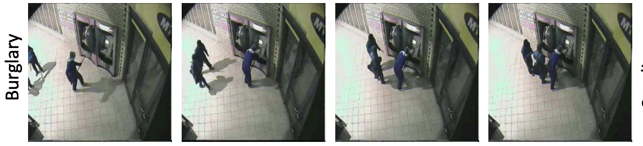
Dimensionality reduction for anomaly detection

• A common application for dimensionality reduction is anomaly or outliers detection. For example:

  • Detecting fraud transactions.

  • Detecting irregular activity in video frames.

  • It’s hard to find good anomaly detection datasets. A popular one is The KDD Cup ‘99 dataset.